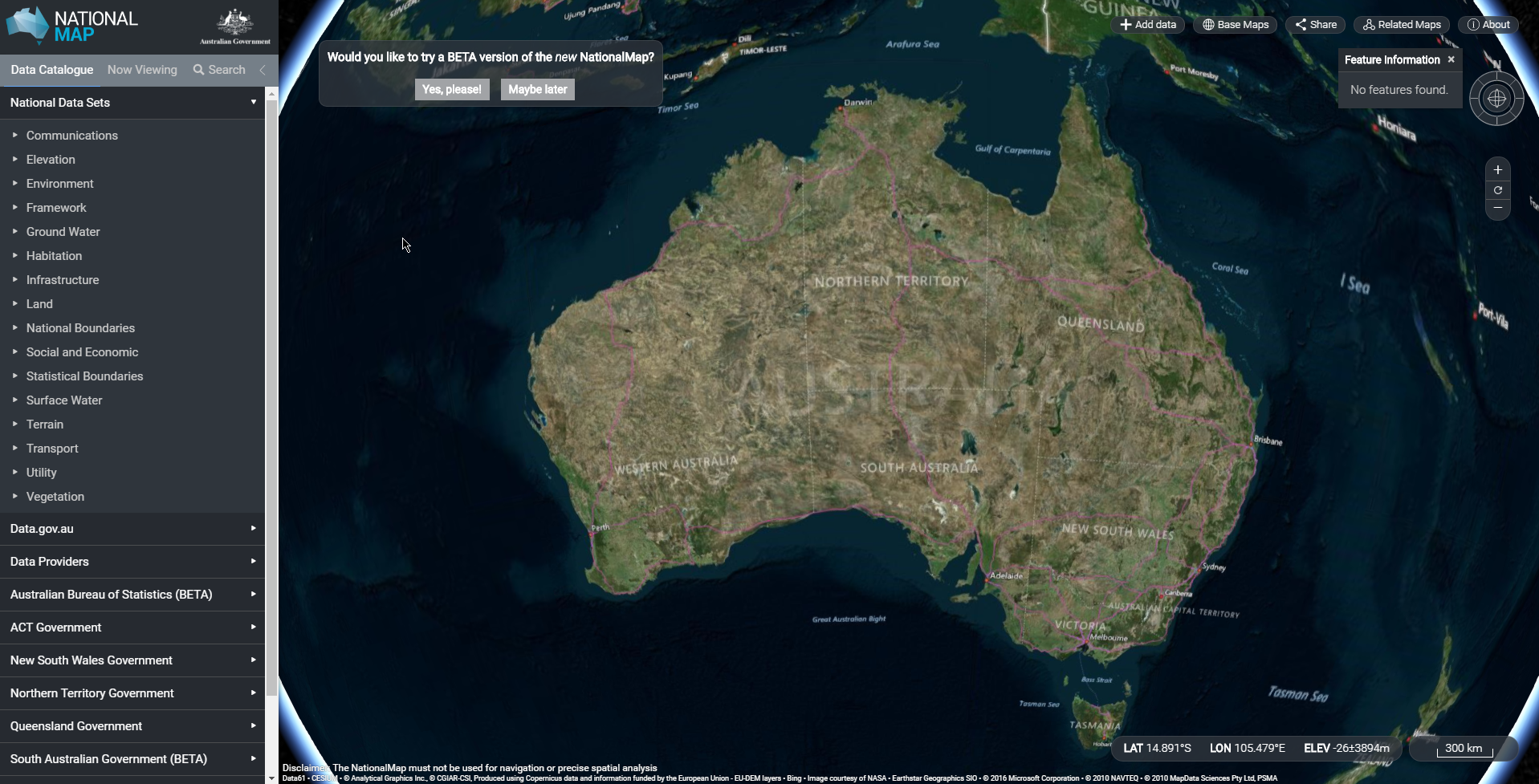
I have been watching a very interesting video on the FOSS4G NA’s YouTube channel by Steve Bennett a software engineer from a company called Data 61 all about their creation and implementation of an opensource website for all geospatial data in Australia. I wasn’t aware of this website and decided to take a look at it, it’s called http://nationalmap.gov.au/. When the interface loads uses Bing as its default basemap.
It has a very impressive range of datasets available to view. A very useful feature is that where available you can download the data directly. The National Map does not host any data directly but ‘provides a federated interface to the diverse servers already operated by the various government agencies, running Geoserver, THREDDS Data Server, ArcGIS Server, CKAN, Socrata, and many more’.
To create the National Map they created a new library called ‘TerriaJS’ that makes it straightforward to build 3D web-based geospatial data explorers. The crucial point to make with TerriaJS is that it is entirely opensource and is already being used by a host of different companies both inside and outside Australia. The road that Steve and his colleagues have traversed has been long with a screenshot of his YouTube video shown below to give the timeline.
Screenshot from FOSS4G NA’ YouTube video
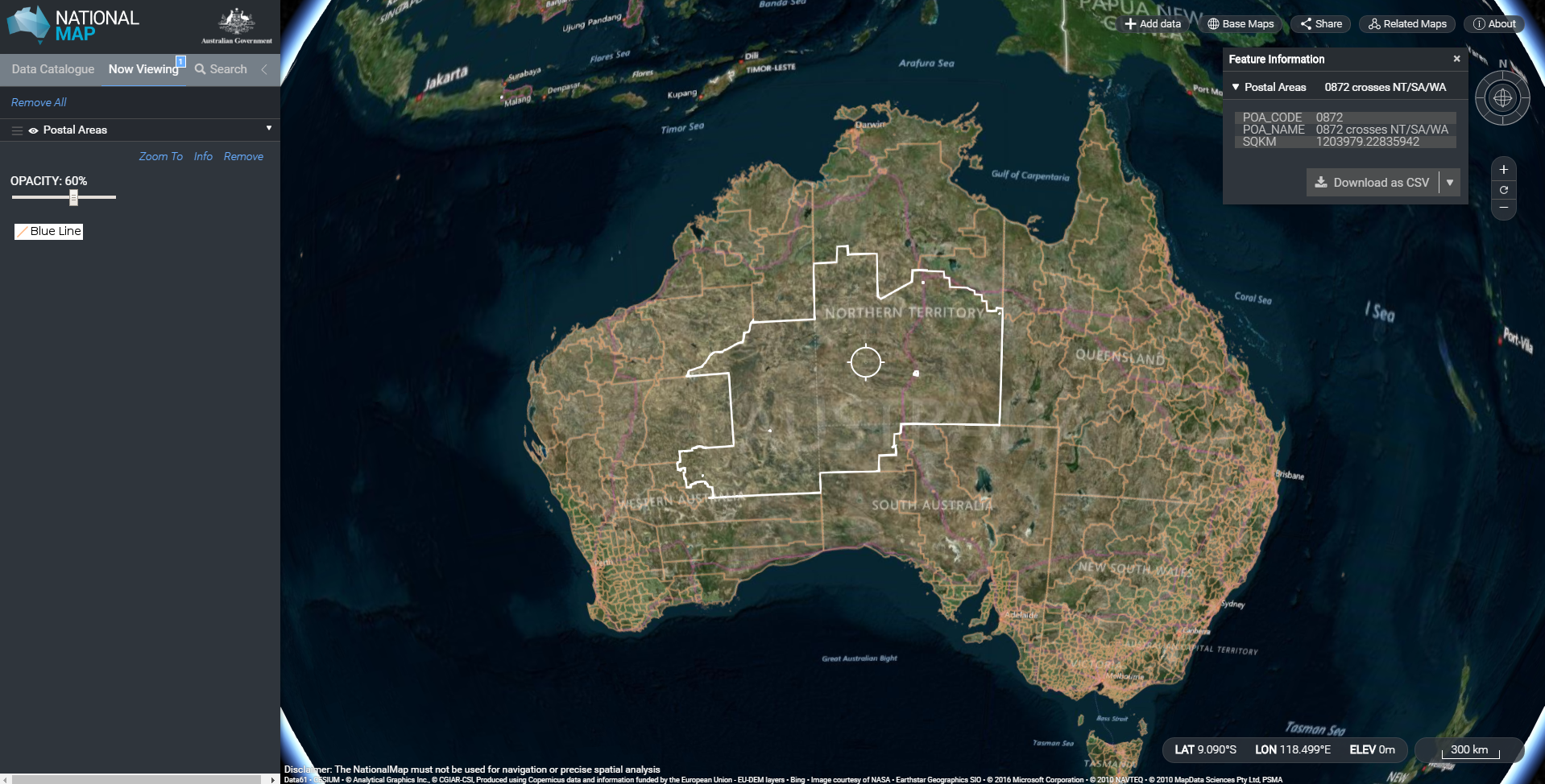
The search function works very well and is very responsive. I searched for and downloaded the Australian post code areas, it worked flawlessly. A screenshot of querying the post code layer is shown below.
Querying the post code layer
Any query can be downloaded as either a CSV or JSON. One post code caught my attention for the sheer size of it at 1,203,979km². To put that in perspective that one post code is over twice the size of France or over 17 times the size of the Republic of Ireland.
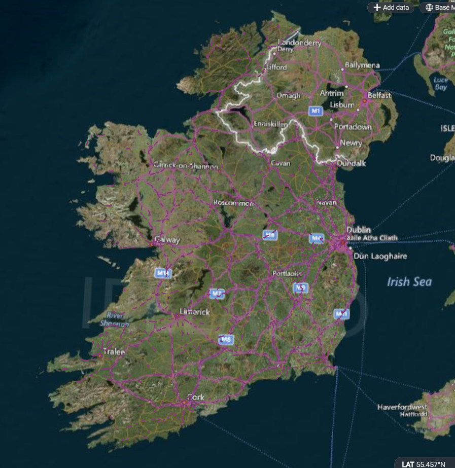
The website has the ability to upload data. I uploaded a JSON file of Irish speed camera zones, it worked flawlessly as shown below.
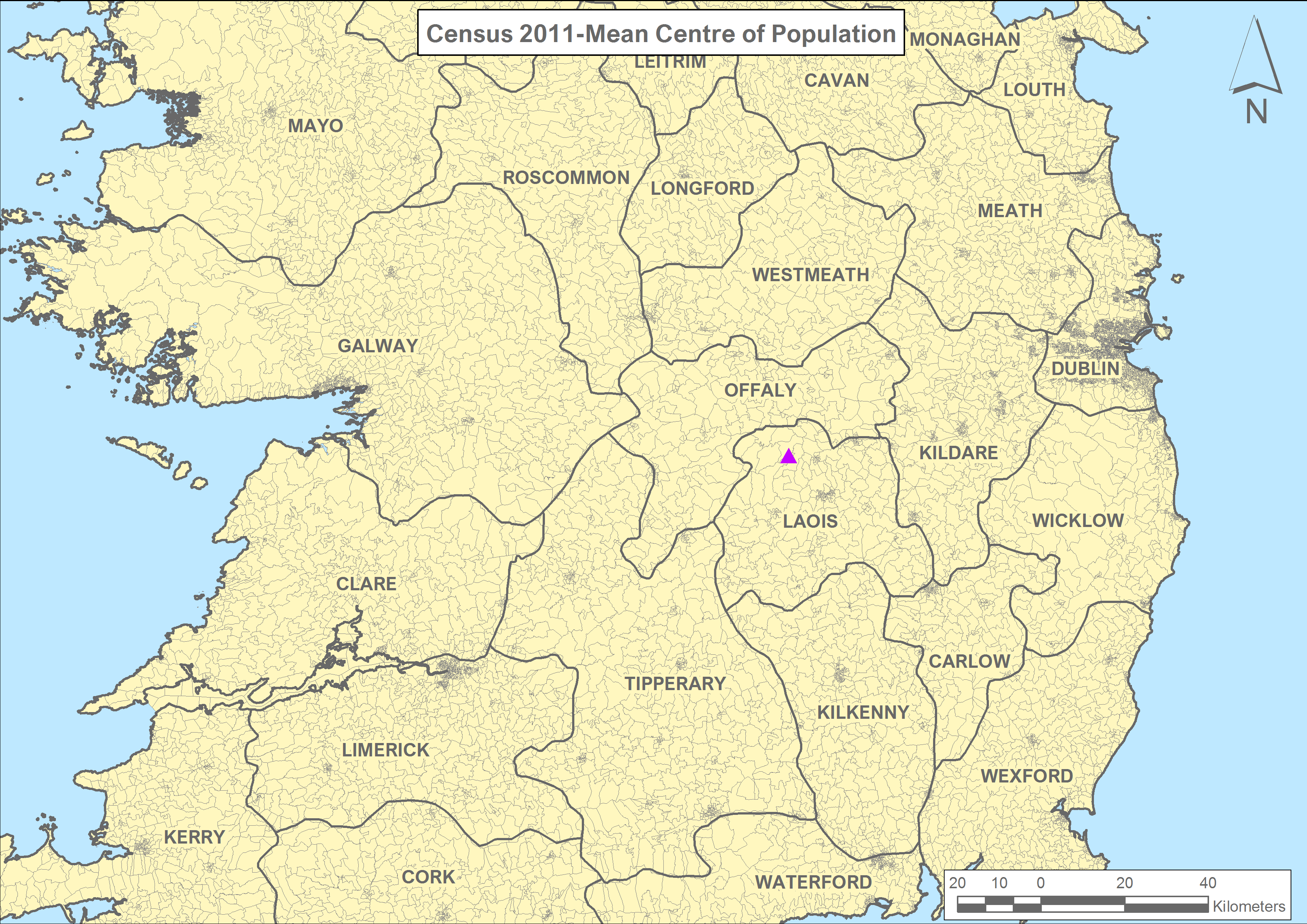
In anticipation of results of the 2016 Irish census I thought that it would be interesting to calculate the mean centre of population from the 2011 census. The data was downloaded from the Central Statistics Office website. The next step was to download the census boundaries from here. Once downloaded they were opened in ArcMap 10.2.2 and the Mean Center (sic) tool was used from the Spatial Statistics toolbox to calculate the mean centre with the total population for each small area used for the weight. Below is the mean population centre for the Republic, it is located in the townland of Capard, Co. Laois.
I recently read Annekatrien Debien’s post on Digital Geography regarding extracting information from Sentinel-1, specifically ship data and I decided to follow the tutorial for an area of the South-West coast of Ireland.
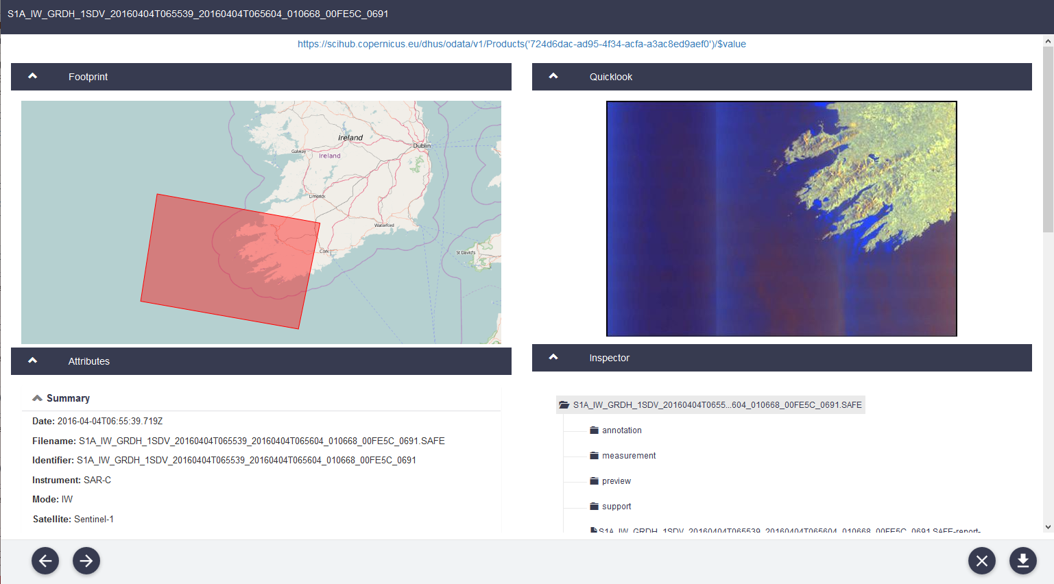
The first step was to download a Sentinel-1 image from the Copernicus website. I downloaded an image captured on the 4th April 2016.
This is the download dialogue box on the ESA Copernicus website.
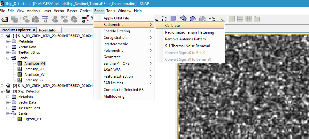
The next step was to open the image in the SNAP toolbox. Once it was opened, the next step was to calibrate the image. You have to go to Radar –> Radiometric –> Calibrate as shown below.
Calibrate Menu Option
To calibrate you have to select both bands VH and VV on the second tab that is displayed after you click calibrate and the parameter you need it Sigma0.
Once the calibration has run then a second product appears in the window.
Extracting Information on Ships:
The next step was to extract information on the ships. The option is located at:
Go to Radar –> Feature Extraction –> Ocean Tools –> Ocean Object Detection
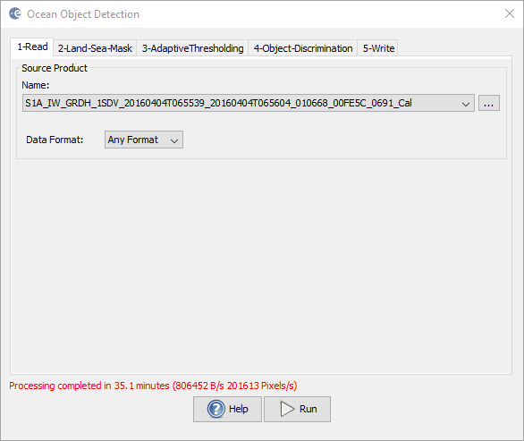
You have to make sure that the calibrated image is the one selected as shown.
Dialog Option
The Sigma0_VH is the band to select. You then click run. It is quite memory and CPU intensive and took my computer 35 minutes to complete (it’s only a few months old with a lot of RAM so that may have helped). It is a very intensive process as you can see below.
Task Manager for Object Detection
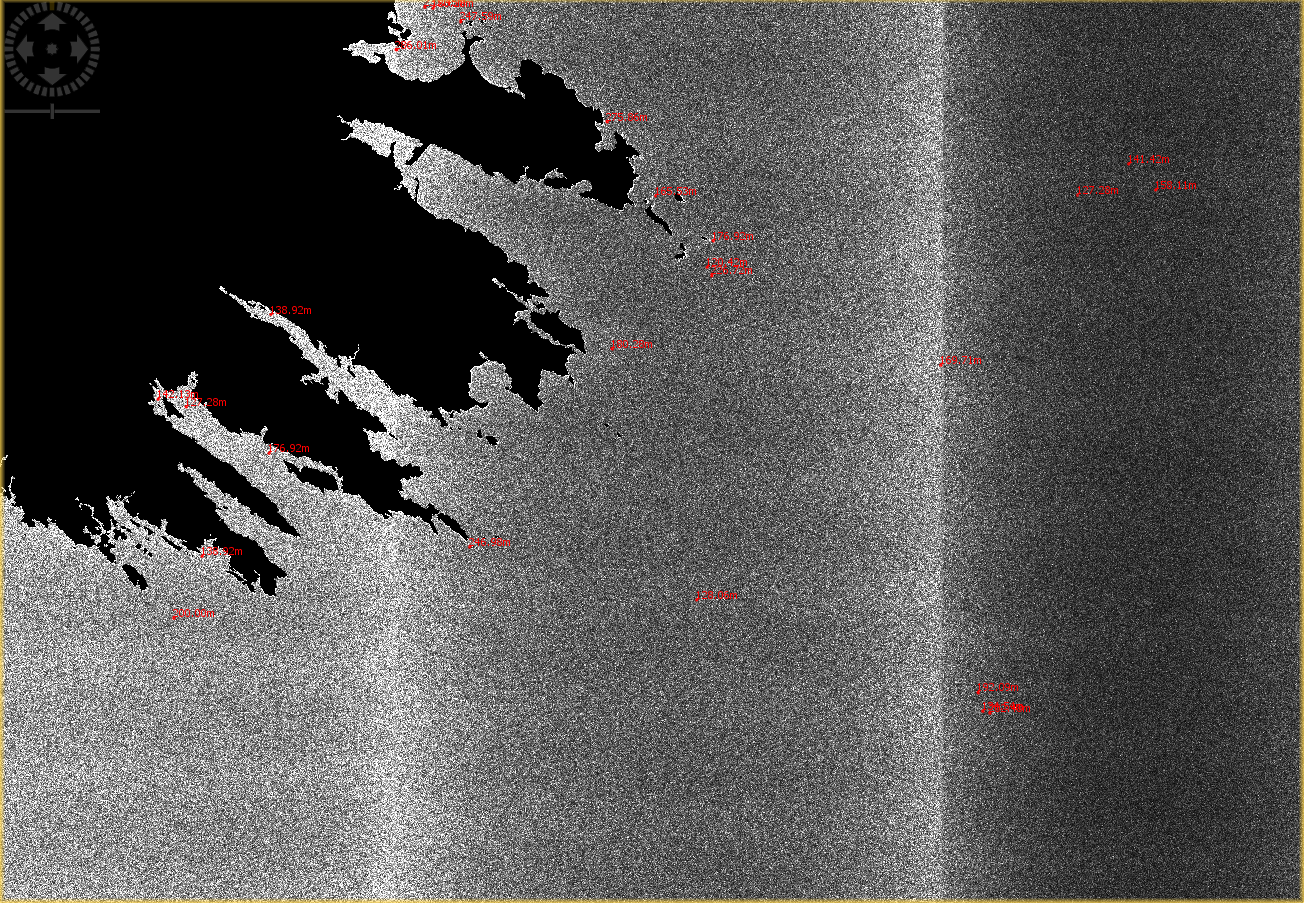
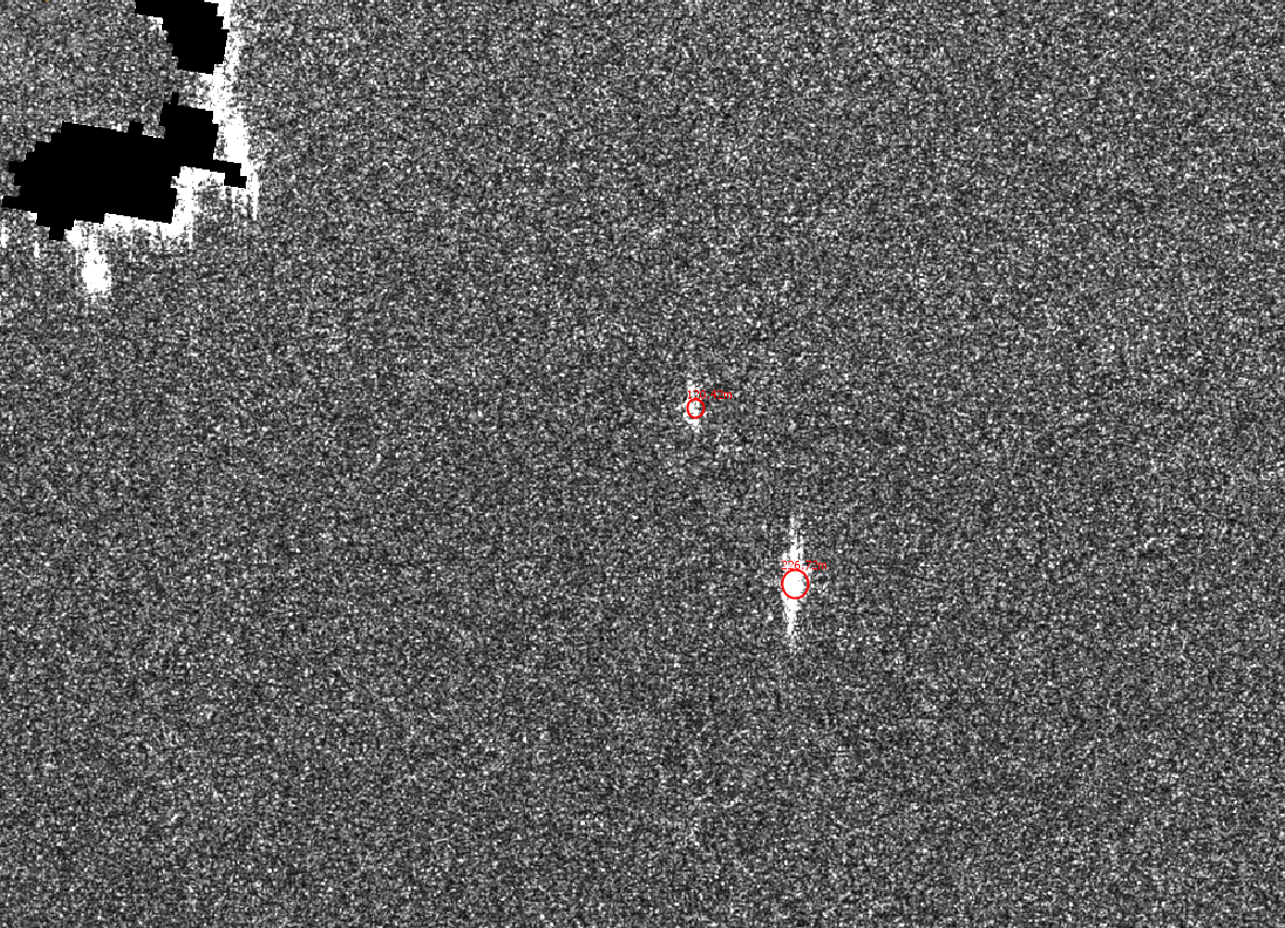
The end result in the SNAP toolbox was as follows:
Ship Detection Results
Individual Ships looks as follows:
Individual Ships in Results Window
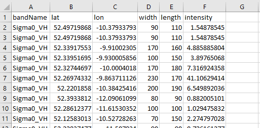
As Anne has desribed on her blog, the next step was to located the log file (xml file) and import it into Excel and save as a CSV as shown below.
CSV File from Excel
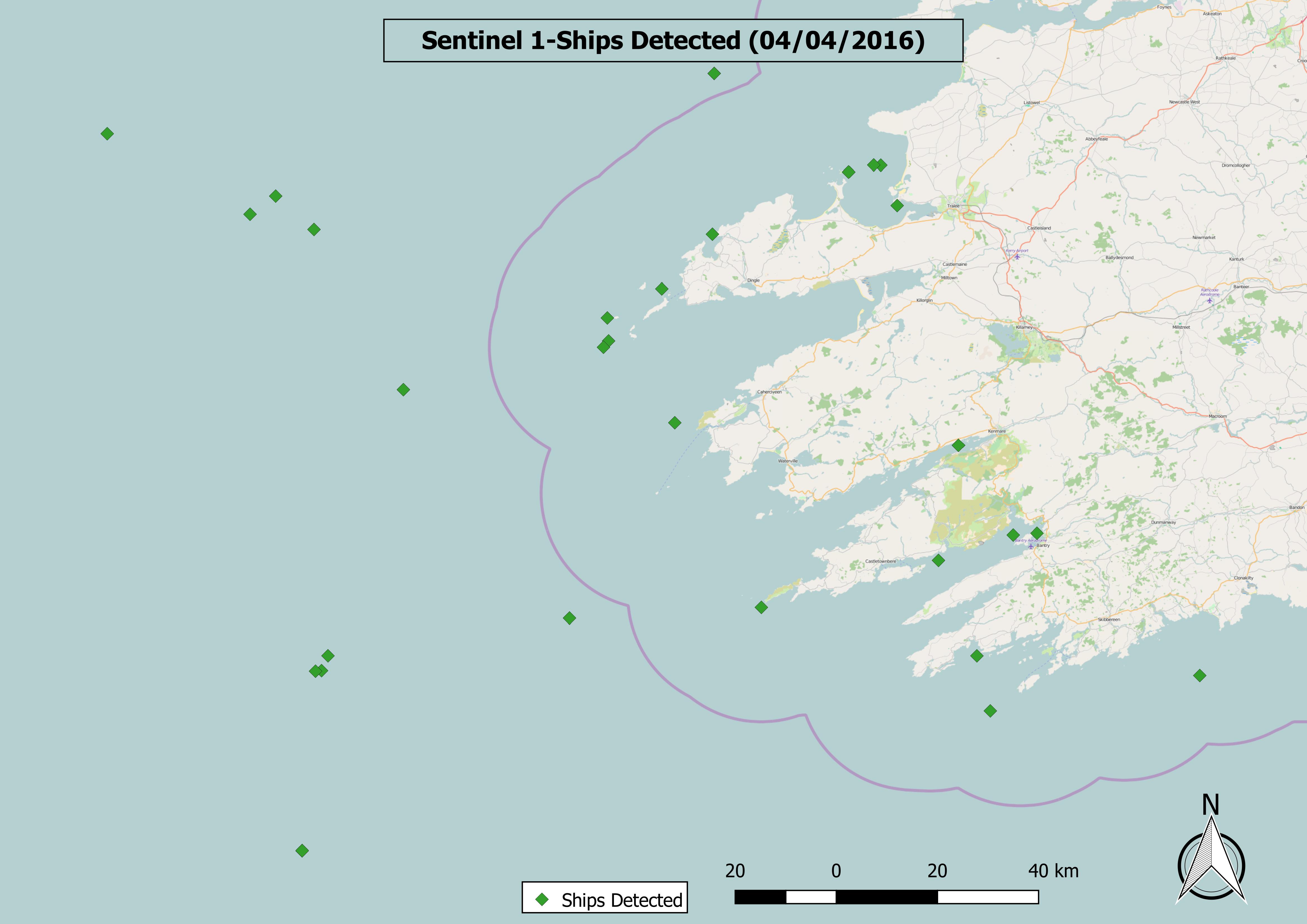
This was then imported into QGIS and a simple map was created with OSM as the background. The end result is shown below:
With a number of Irish data sets having been made available under the Creative Commons Attribution 4.0 license I thought it would be interesting to take a look at one of these, the Sites and Monuments Record (SMR) from the National Monuments Service. This falls under the Archaeological Survey of Ireland which is a unit of the National Monuments Service. It basically records any known monuments from mainly pre-dating AD 1700 and some from the post-AD 1700 period.
I very briefly queried this database online using the ESRI web-app which limits the number of visible records to less than 1000. The next step I did was to download each county’s shapefile individually (as the entire country cannot be downloaded together). Once these were downloaded as 27 different shapefiles the next task was to merge them into one. The easiest way to merged these was to use the Geospatial Data Abstraction Library (GDAL). The easiest and most convenient way to install this is to use the OSGeo4w installer that takes the hard work out of it. It is available from here. Once this is downloaded and installed (I chose the express install and only installed GDAL.
I had the 27 shapefiles in a folder on my desktop called ‘National Monuments’. I opened the OSGeo4w shell and changed the directory to the National Monuments folder and made a new directory within called ‘merged’. The following script was then run:
C:\>cd C:\Users\Donie\Desktop\National_Monuments

C:\Users\Donie\Desktop\National_Monuments>mkdir merged

C:\Users\Donie\Desktop\National_Monuments>for %f in (*.shp) do (
More? if not exist merged\merged.shp (
More? ogr2ogr -f "esri shapefile" merged\merged.shp %f) else (
More? ogr2ogr -f "esri shapefile" -update -append merged\merged.shp %f -nln Merged )
More? )
The result of the above was a merged shapefile of all 27 of the other shapefiles. As this was a huge shapefile with approximately 150,000 entries the next step was to create a PostGIS database and import the shapefile. Using pgAdmin III a postgres database was created called ‘National’ and a postgis extension was created using the following line of code:
create extension postgis;
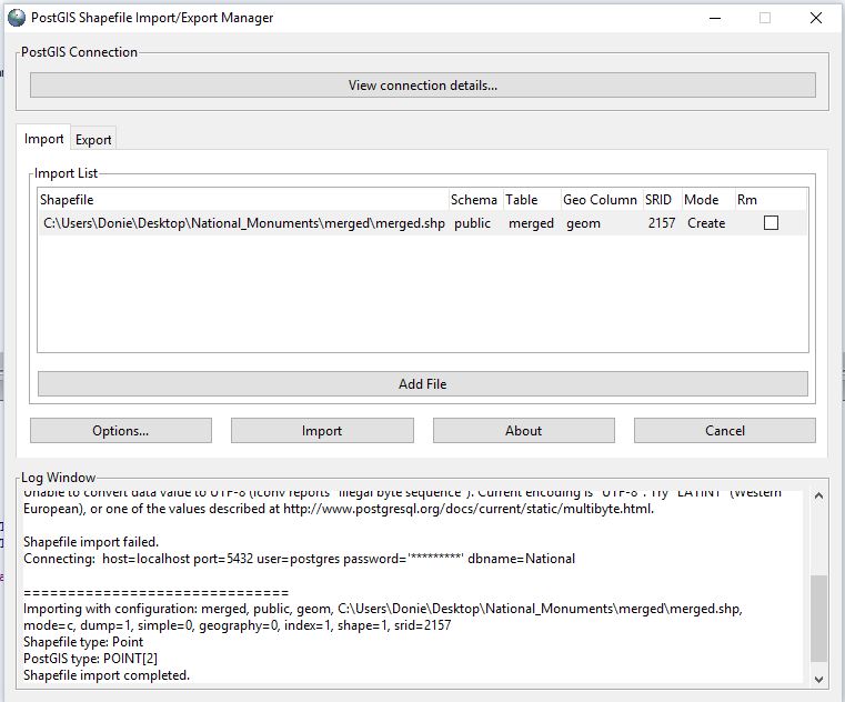
The next step was to import the shapefile, this was completed using the PostGIS Shapefile Import/Export Manager. Only two items needed to be changed, the Spatial Reference System Identifier (SRID) was changed to 2157 (Irish Transverse Mercator) and the character encoding was changed to ‘LATIN1’.
The next step was to query the data to see what needed to be removed/edited. A simple SQL statement was run to select everything in the database:
SELECT * FROM merged;
From this 153,364 records were returned and it was clear that the column ‘classdesc’ was the column needed to find all data on ringforts. The data was then ordered using the following:
SELECT * FROM merged
ORDER BY classdesc;
From examining the associated online data there are four types of ringforts that I need to export:
Ringfort – rath
Ringfort – cashel
Ringfort – unclassified
Enclosure
The easiest way to do this was to create a new table with just those records in it and export these as a new shapefile. The following SQL script was used to create the new table:
CREATE TABLE ringforts AS
SELECT classdesc
FROM merged
WHERE classdesc IN ('Ringfort - rath', 'Ringfort - cashel', 'Enclosure', 'Ringfort - unclassified');
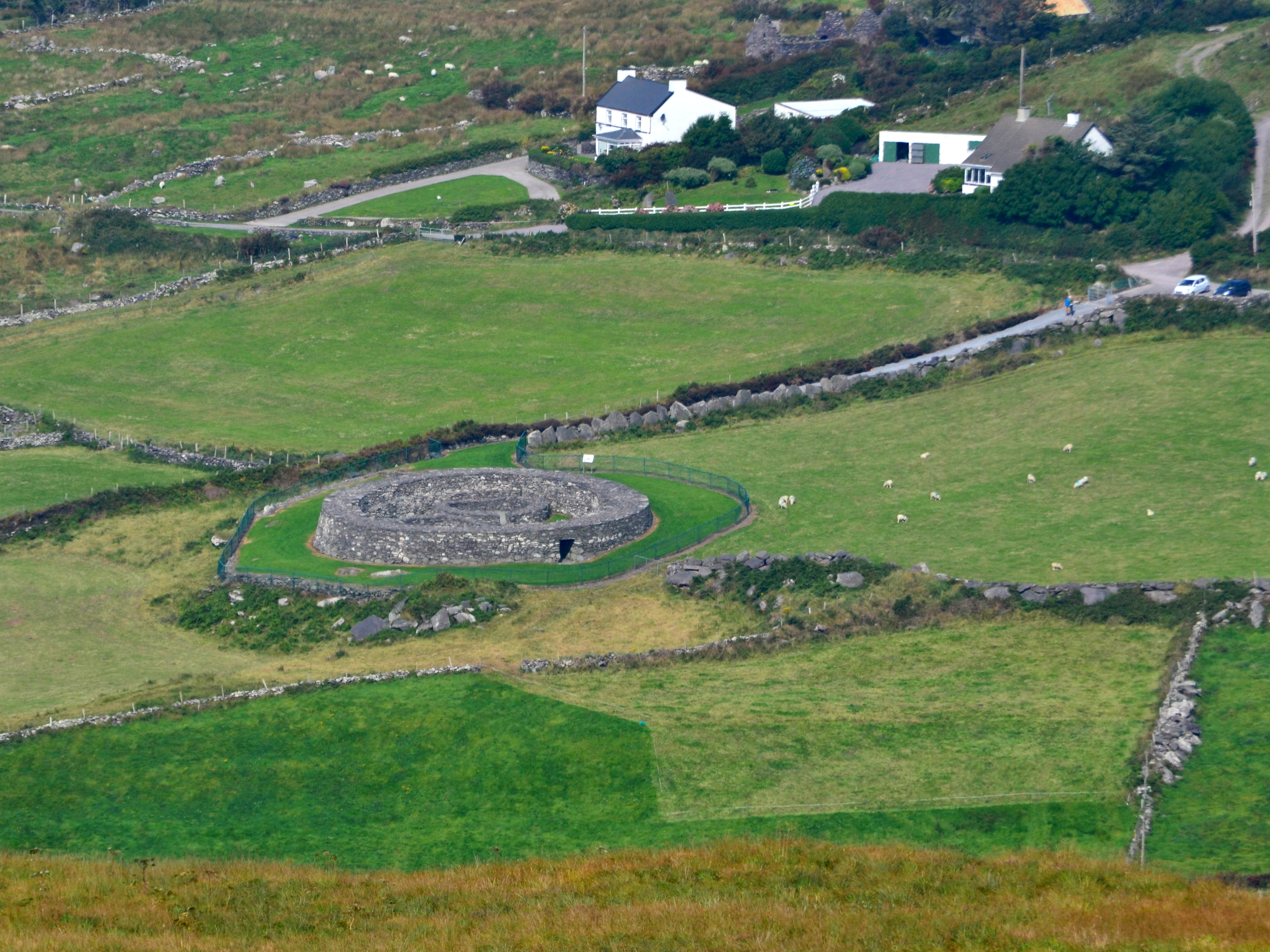
Once this new table was created it was exported to a GeoJSON file using the ogr2ogr. The following was the code used:
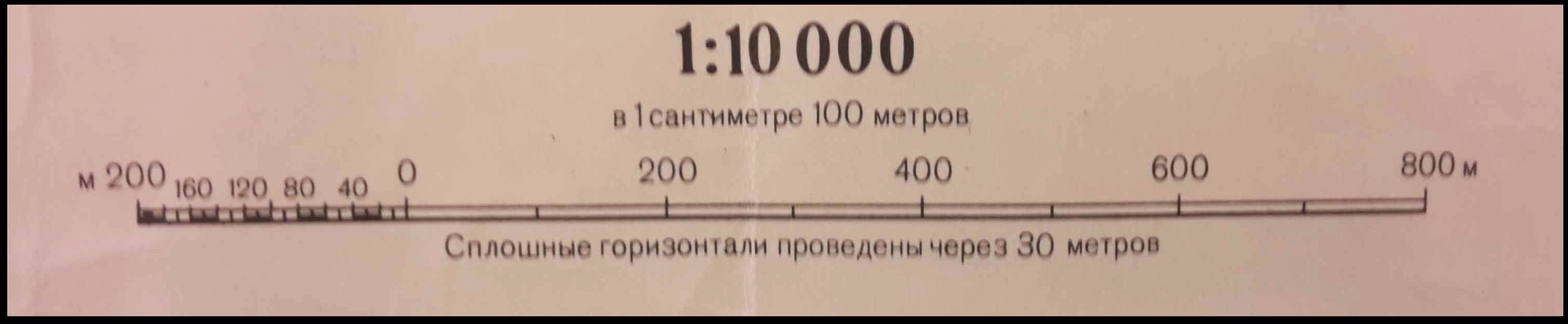
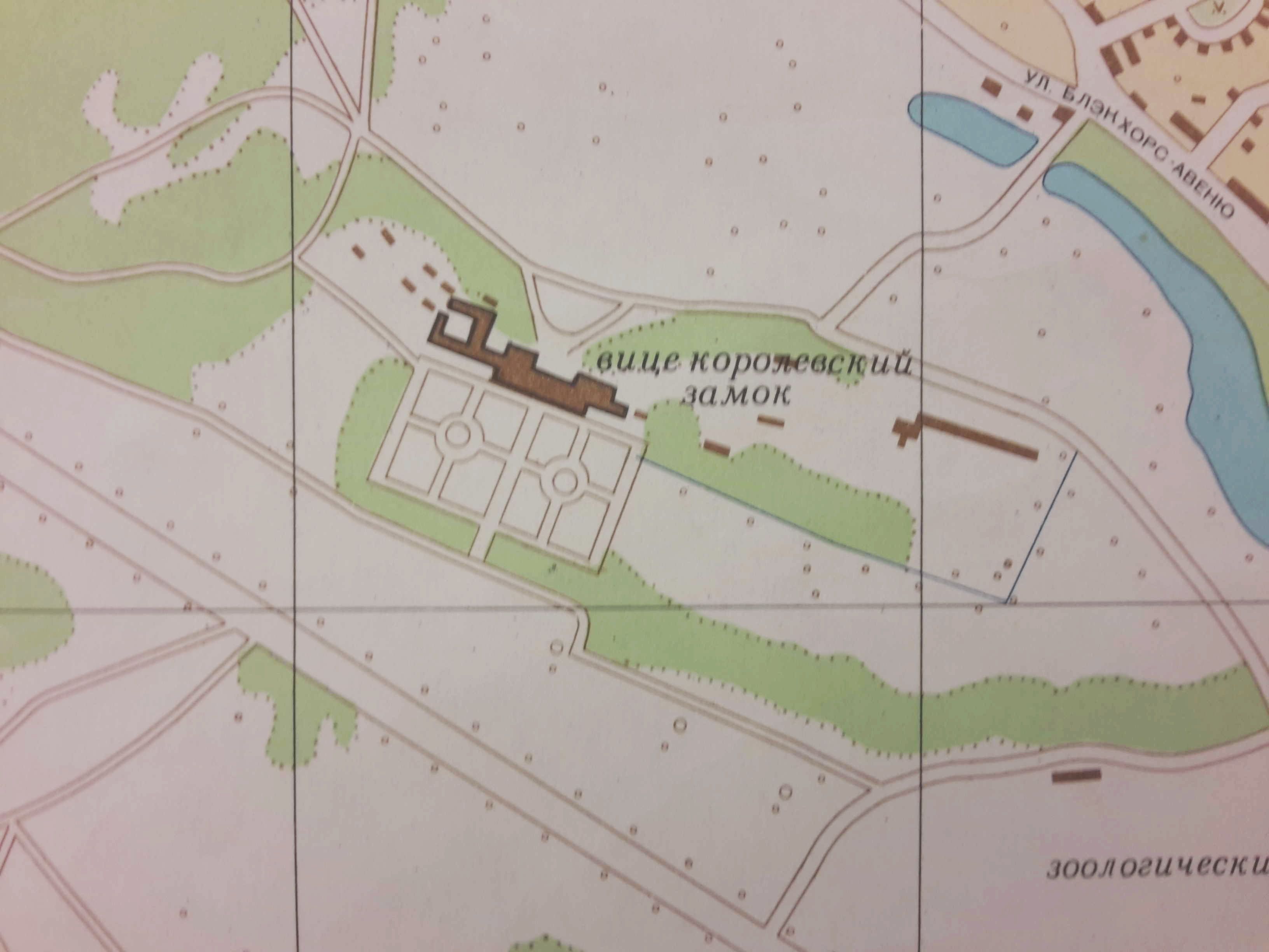
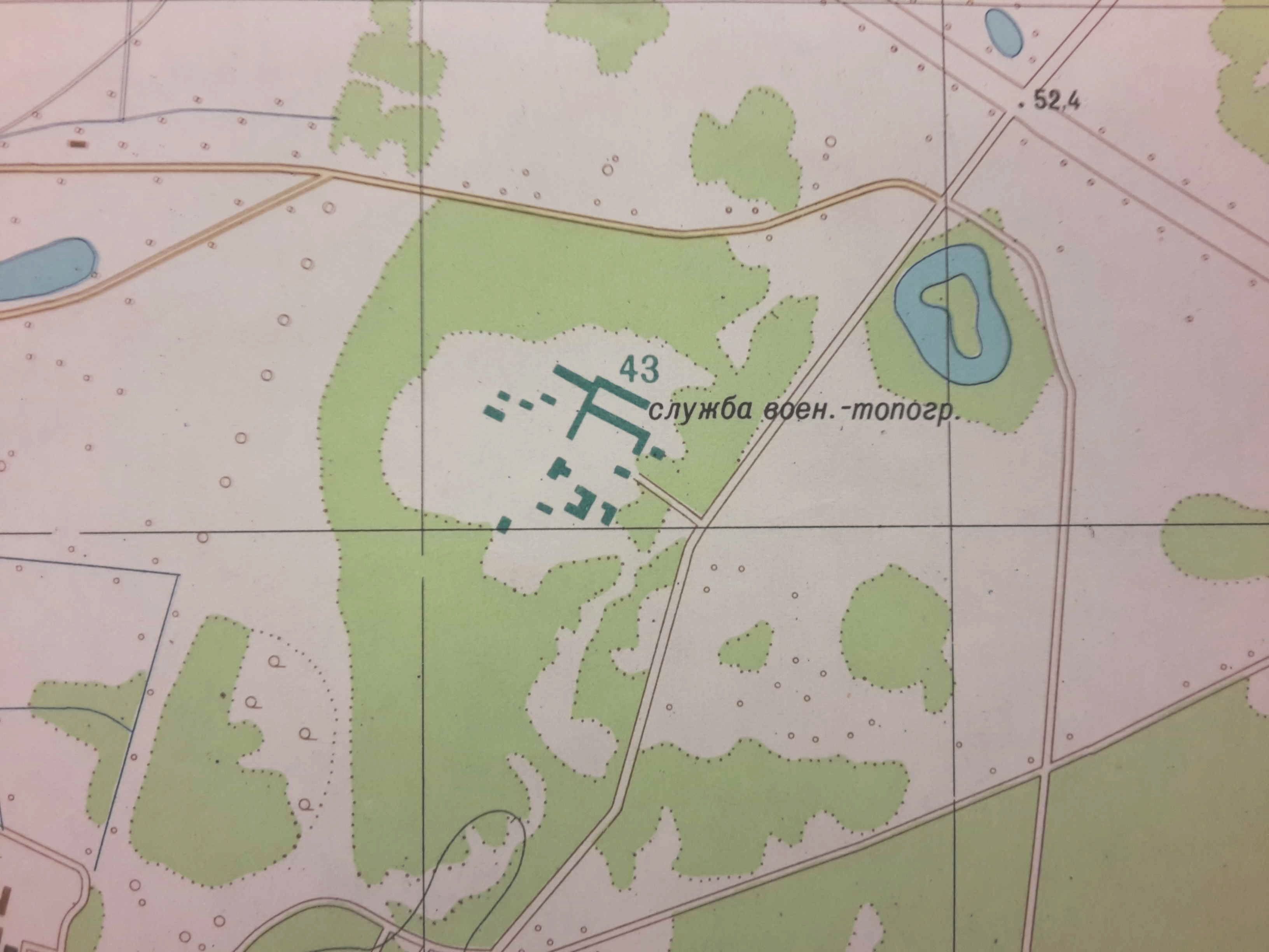
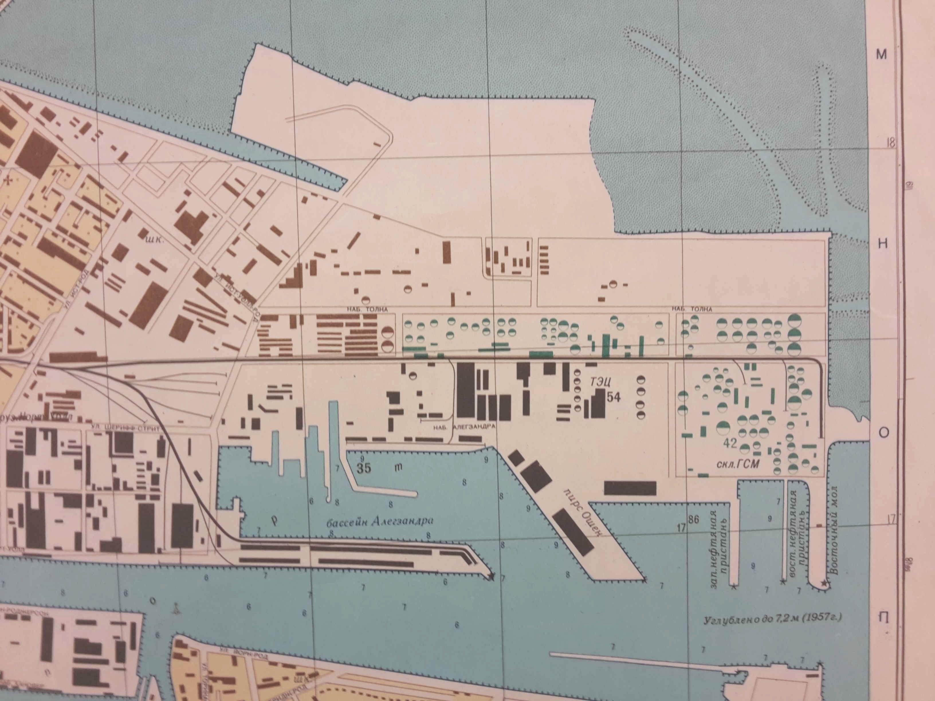
Recently, I’ve been reading about the maps that the Soviet’s produced of major cities in the United States, the UK and Ireland. Being Irish I was interested in what they had completed for Ireland. After some searching online I managed to get my hands on an original copy for Dublin. It was produced in 1980 at a scale of 1:10,000.
1,10,000 map of Dublin published in 1980.
These maps were originally created to provide information should they ever decide to invade Ireland. They were created at the height of the cold war, 1980 was the year that the US boycotted the Olympics in Moscow and Tito died in Belgrade. With this in mind I started looking at the different locations in Dublin that I would be interested in should I have decided to invade.
The map includes Áras an Uachtaráin (The official resident of the President of Ireland) as shown below. The layout of the building and the ground hasn’t changed much in the past 36 years.
Áras an Uachtaráin-The official residence of the Irish President.
It would make sense that if you were making covert maps to be used by your military that you would know the location of the national mapping agency of a country you might invade. In this case they also shared my sentiments, the Ordnance Survey of Ireland (OSI) has been included in purple.
Ordnance Survey Ireland Headquarters, Phoenix Park
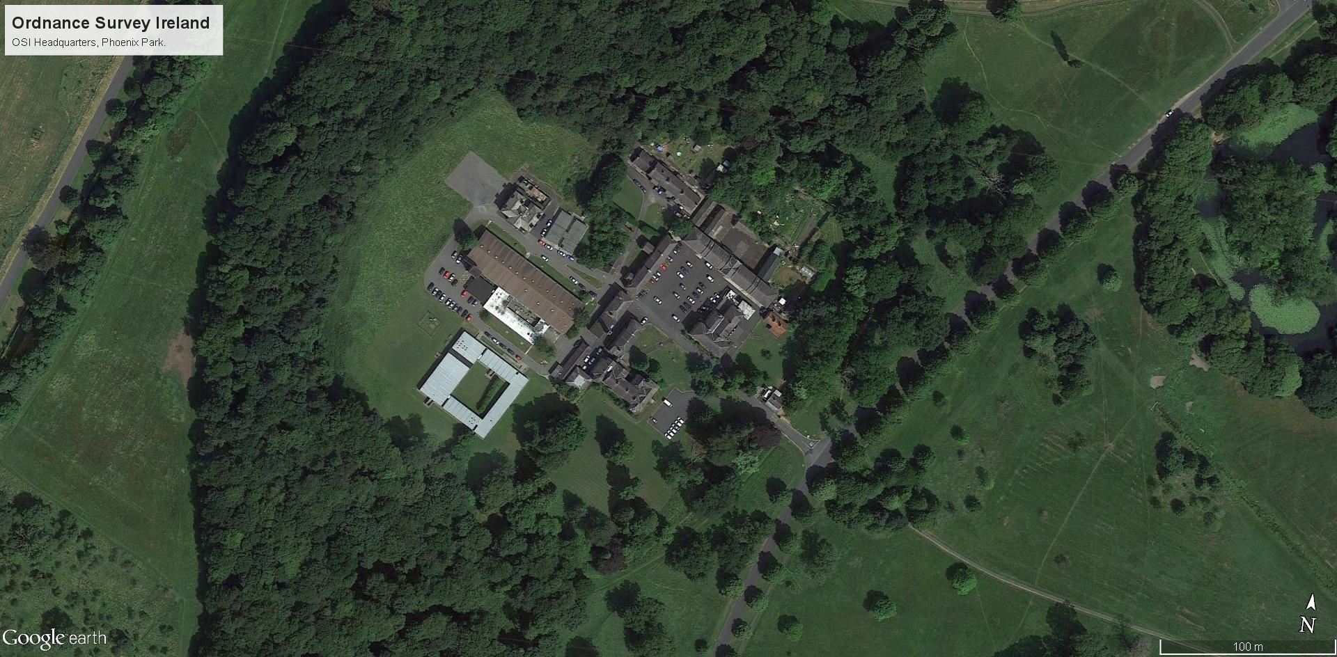
Searching for maps of the Phoenix Park from 1980 proved fruitless (at least for the time being, I will be in Dublin in March and I shall try again). I have to think that even with the buildings they have included that they left out a lot of outlying buildings. Below is the OSI as it looked on the 7th of December 2013.
OSI, Phoenix Park, Dublin. Captured, 07/12/2013.
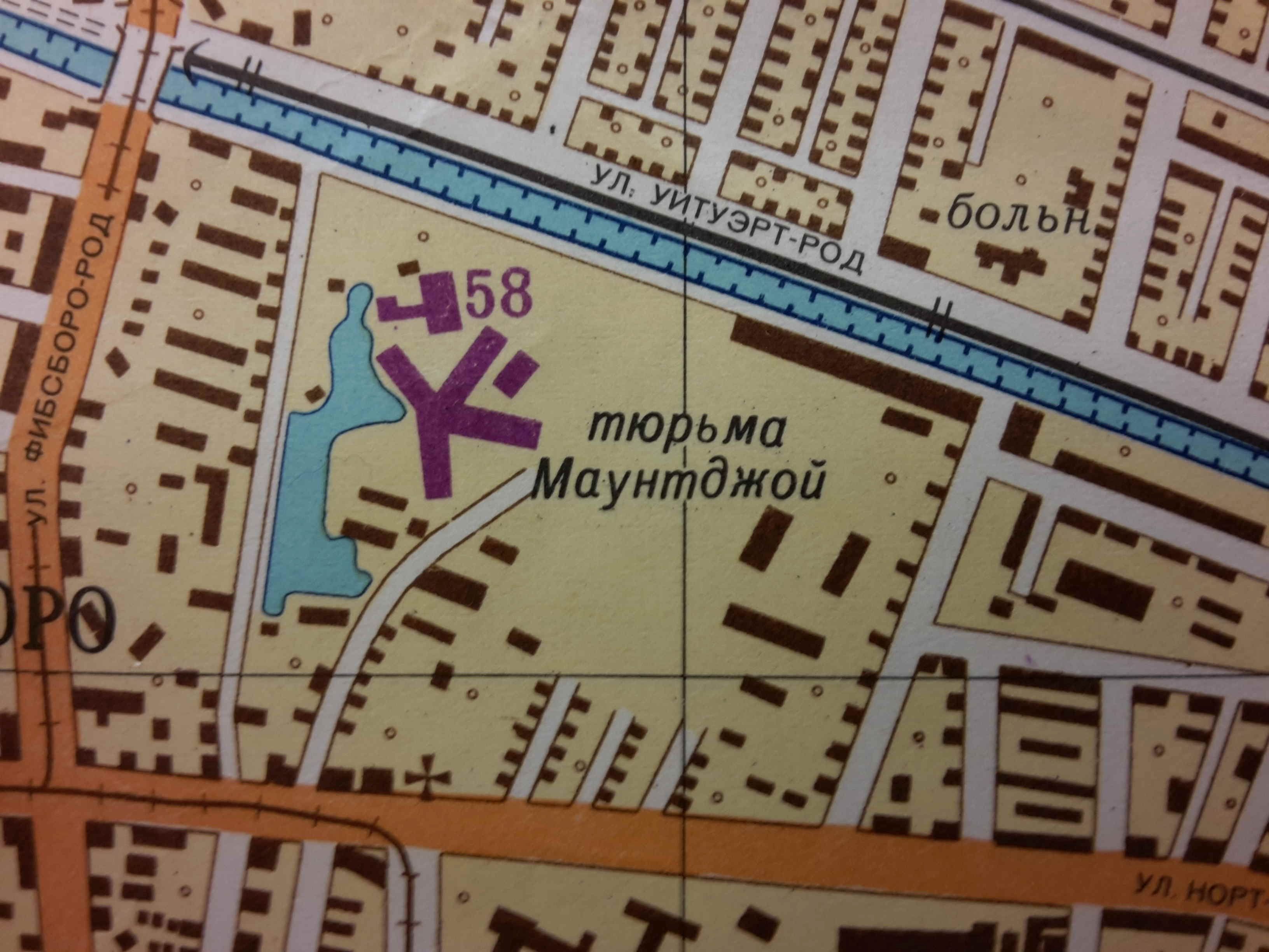
The level of details for the rural areas is quite sparse even at 1:10,000 but for the city another building that they mapped was Mountjoy Prison. This prison was opened in 1850 and its design was based on Pentonville Prison.
Mountjoy Prison, Dublin.
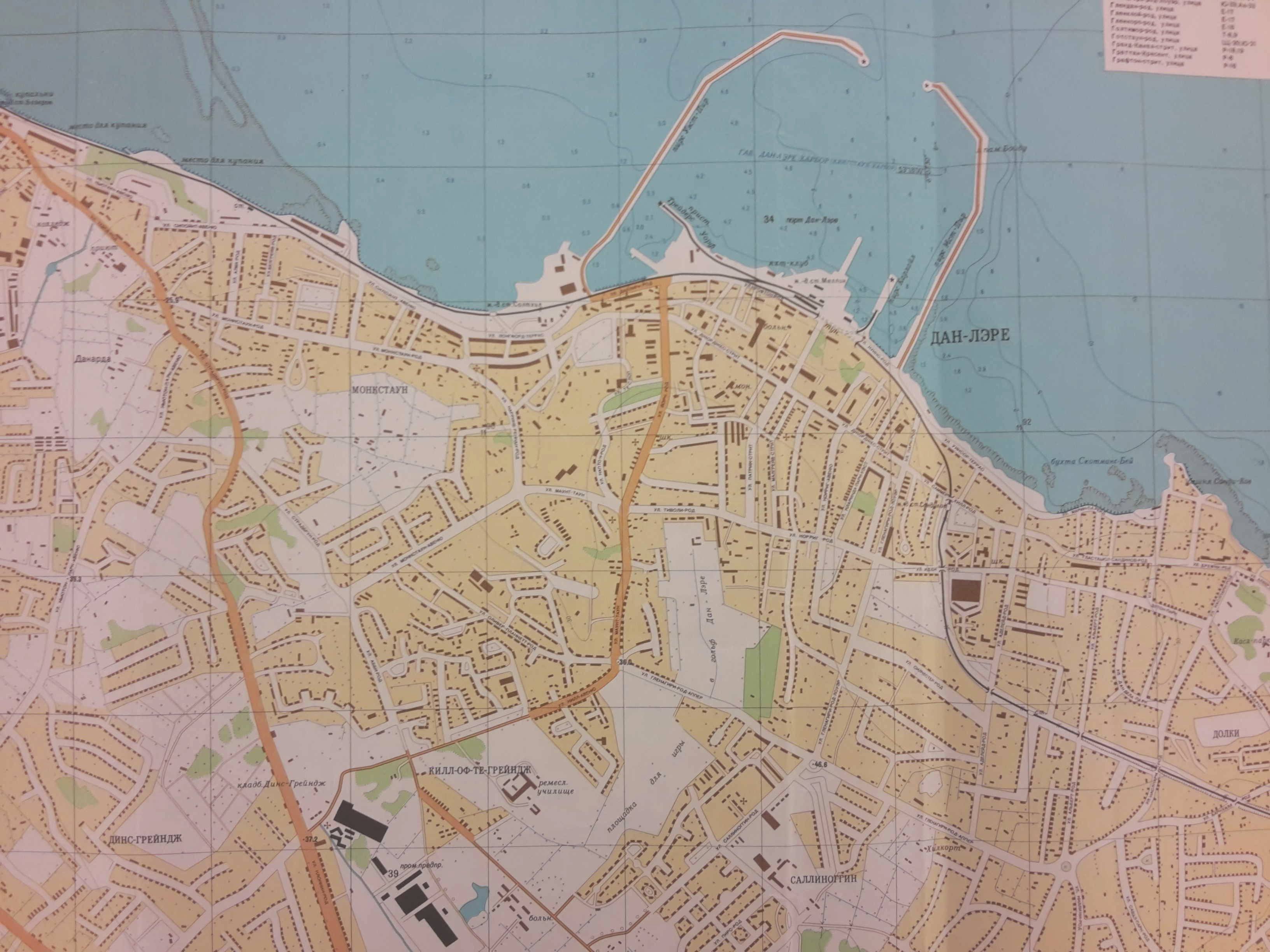
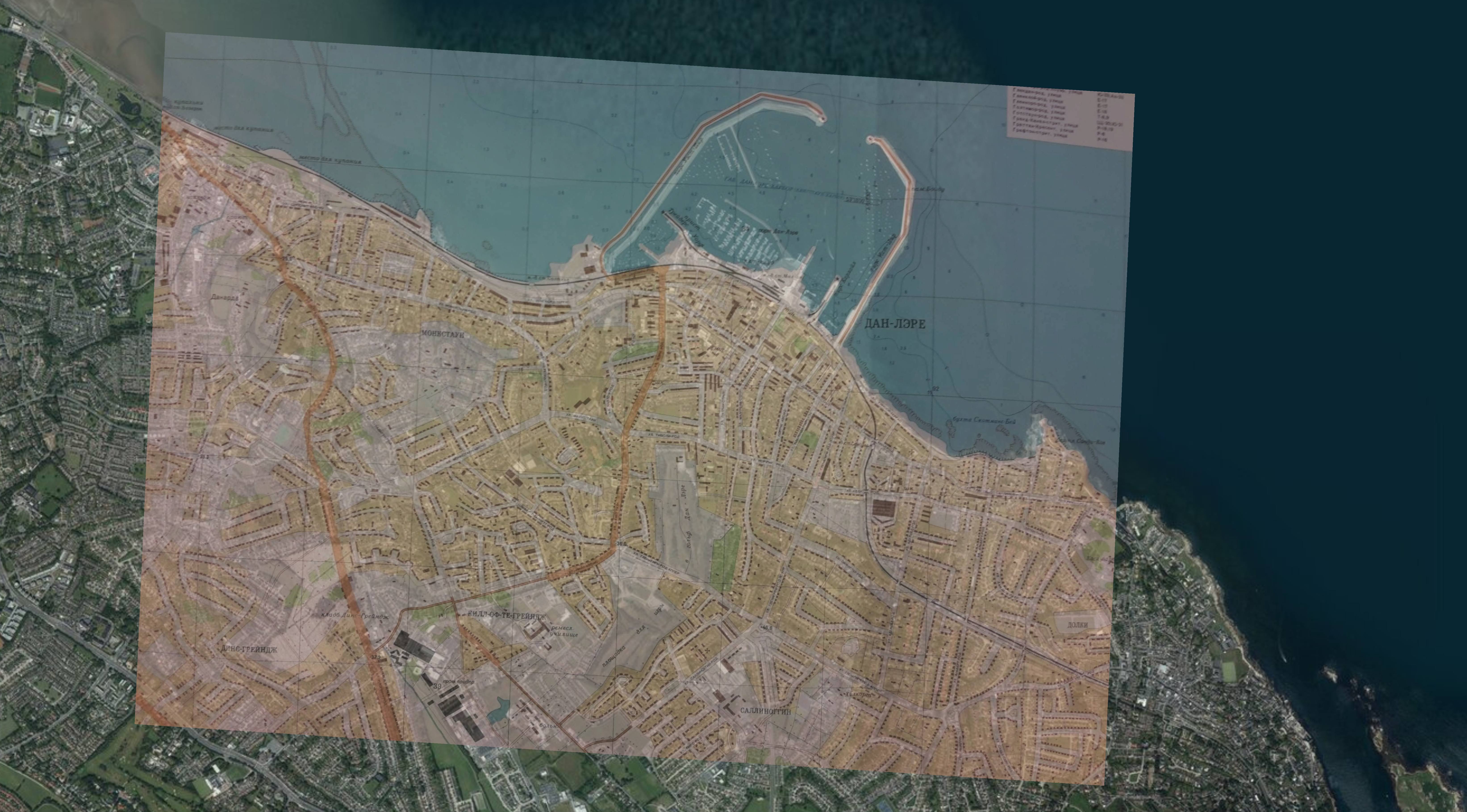
Below is shown what the prison looked like in the 7th of December 2013. I was not impressed (even for 1980) of the cartographic standard of this series of maps of Dublin. There is very little details shown below. The street symbology follows no hierarchy, the labeling is inconsistent and poorly executed and there is virtually no detail on buildings, save for the odd ( and worryingly uniform, even taking into account the large percentage of semi-detached dwellings in this area). To prove the point, I georeferenced the section of the map that I had and overlaid it on satellite imagery. The results are shown below, as usual, hospitals, railways and industrial areas are well marked but residential detail is sorely missing.
Georeferenced-Dún Laoghaire
Albeit crude, the above image gives a good idea of what the Russians were missing out on in Dún Laoghaire. I have checked their coordinates the mount of the harbor and they are accurate (I didn’t doubt this, I thought it was just fun to check!). The last image I’m going to show from this quick look at Dublin is the docks, specifically, Grand Canal Dock and the Ringsend Area. As they would most likely have used Ireland a staging post to invade the UK, they went to considerable lengths to get the dock and the hydrography correct as shown in the image below where almost every building of strategic consequence is mapped.
Dublin Port, 1980.
I hope to update this most when I can source OSI maps from circa 1980.