Recently I finished reading Saroo Brierley’s book, A Long Way Home and titled Lion in the feature film. In it he recounts his extraordinary life story of getting separated from his brother at a train station whose name began with ‘B’ a few hours from home in rural India in 1987. He was five years old and his brother Guddu had taken him the few hours from home to make some extra money sweeping out trains. Guddu leaves him on a bench in the train station to get some sleep while he goes to work. The young Saroo wakes a little later but can find no trace of Guddu, in his panic he hops on a train looking for Guddu, the doors shut and he (over what he believes to be 12-15 hours) ends up in Kolkata (then Calcutta). Here, against all odds he survives on the streets and eventually ends up being adopted by (from the sounds of it) a wonderful couple in Tasmania. In his 20s he begins trying to find his mother and siblings in India by using Google Earth to pinpoint both the town he boarded the train and in turn his hometown.

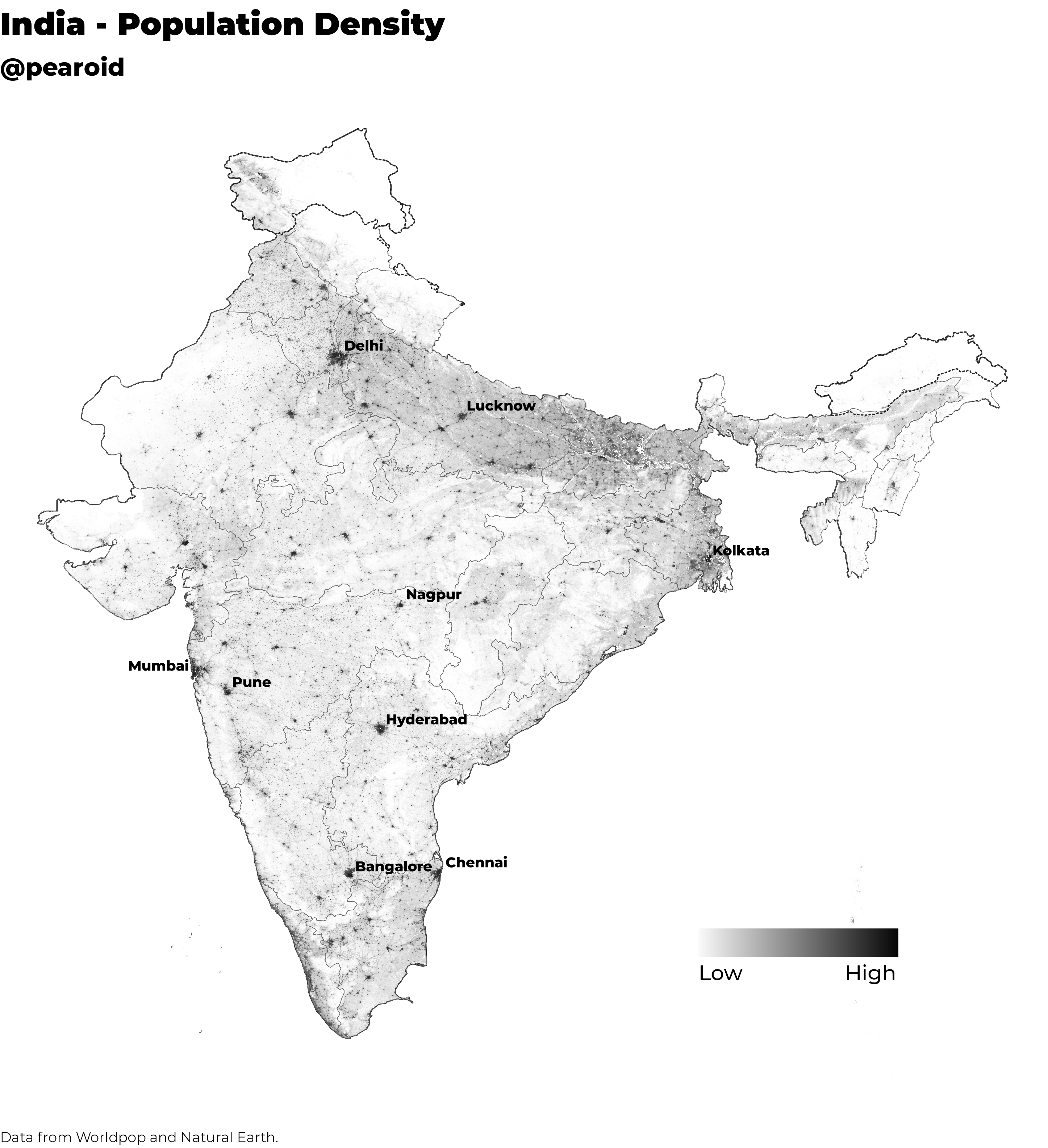
His task was an unenviable one, India is the second most populous country in the world with 1,367,139,484 people (17.5% of the world’s population, Wikipedia). Below is a population density map of India to give some context as to how the population is distributed. These figures are from present day, the population of India in 1987 when Saroo became lost was 819,800,000.
The whole story piqued my interest and I wondered if we were to try the search today using the benefit of open data and open-source software could we make it more efficient. I would like to heavily caveat what is to follow by stating that I am using software and data that would not have been as extensive, complete or fully-featured when Saroo began his search in 2011.
I kept very careful notes whilst I was reading the book and below is an exhaustive list of the criteria that he would follow from his recollections from his five year old self. The criteria is both from his hometown and the town that began with ‘B’ where he got on the train that eventually took him to Kolkata.
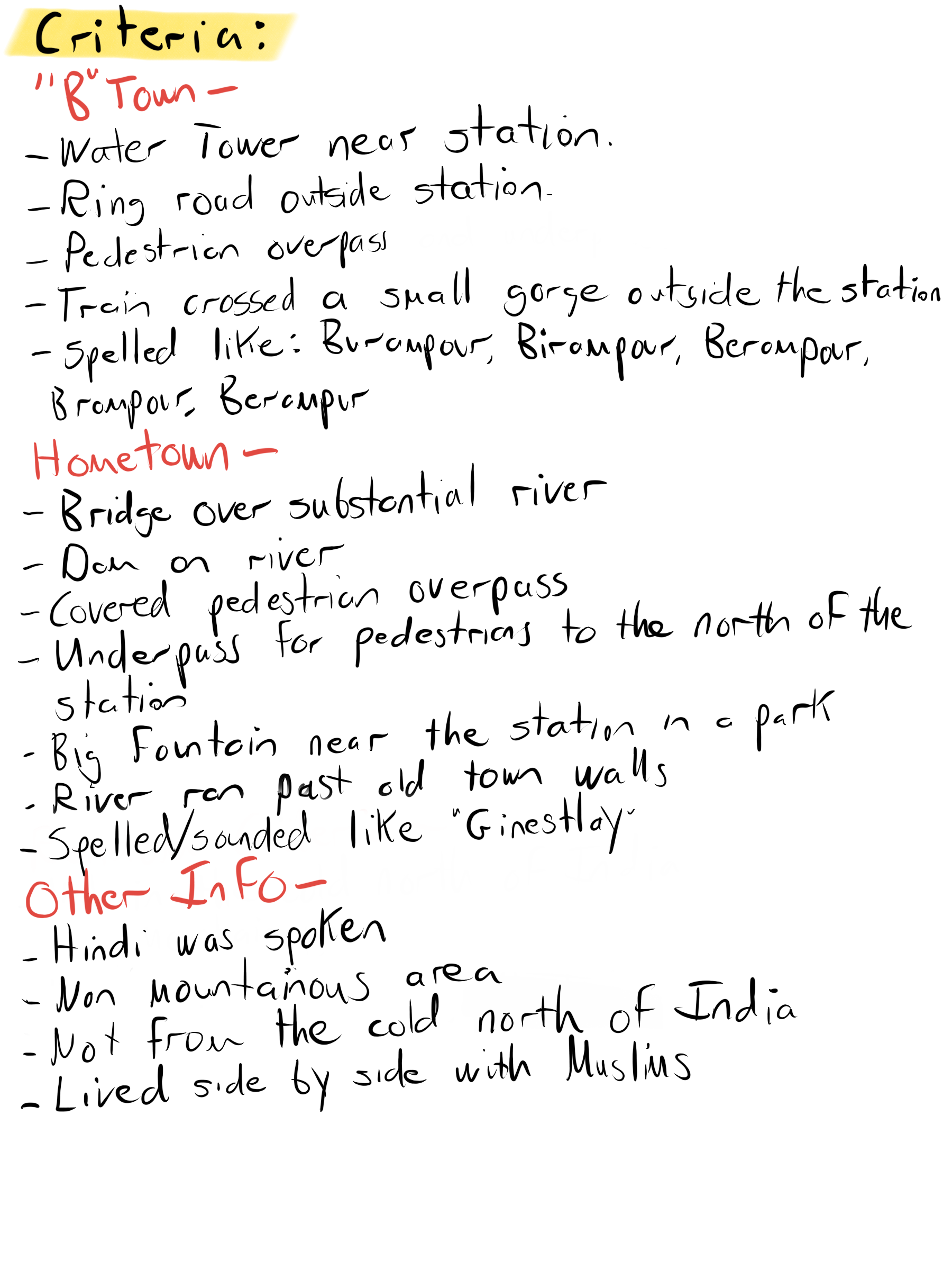
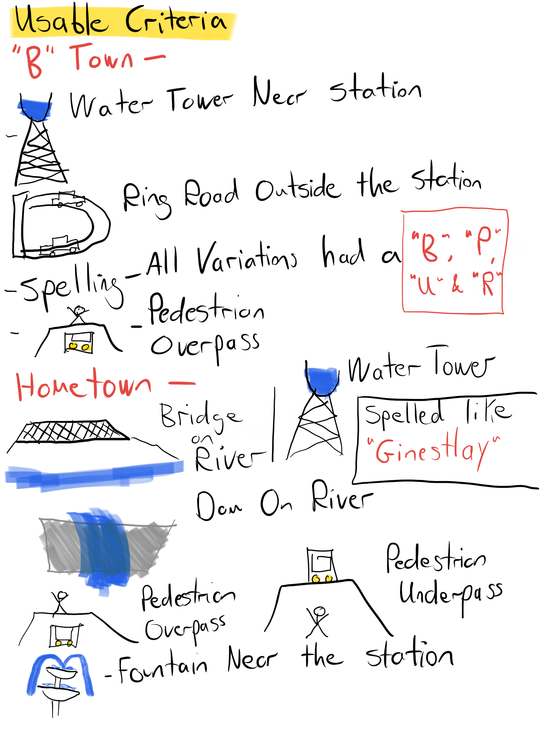
From the initial criteria above it became clear that a number of the criteria would not be usable in replicating the search; such as that it wasn’t in the colder north of India (too subjective) or that they lived side by side with Muslims (a common occurrence in India). Below is a refined list of criteria that I am going to use in order to try and replicate the search.
Saroo’s methodology started with tracing his steps backwards from Kolkata. He knew he got on the train at a station that sounded like ‘Berampur‘ and he thought he was on the train for approximately 12-15 hours. Based on this, he consulted Indian friends of his at college about how to start searching. One friend in particular, Amreen whose father worked for the Indian Railway in New Delhi proved helpful. Her father made an educated guess that trains in India in the 1980s travelled at between 70kph-80kph. Based on this Saroo calculated that he would have travelled 1,000km in that time. He started searching methodically outwards from Kolkata to try and find the station that began with ‘B’ and hopefully, then, his hometown that was about an hour away from this.
If I was to try and recreate the search for Saroo’s hometown, I would need access to as much free geographical data as possible so I turned to OpenStreetMap and specifically the downloads available from Geofabrik. I downloaded the Protocolbuffer Binary Format (PBF) file of the entire of India. The first items I was interested in were the railway lines and railway stations of India. QGIS can load the PBF files natively but the entire of India is a bit of a stretch for it regardless of computing power available.

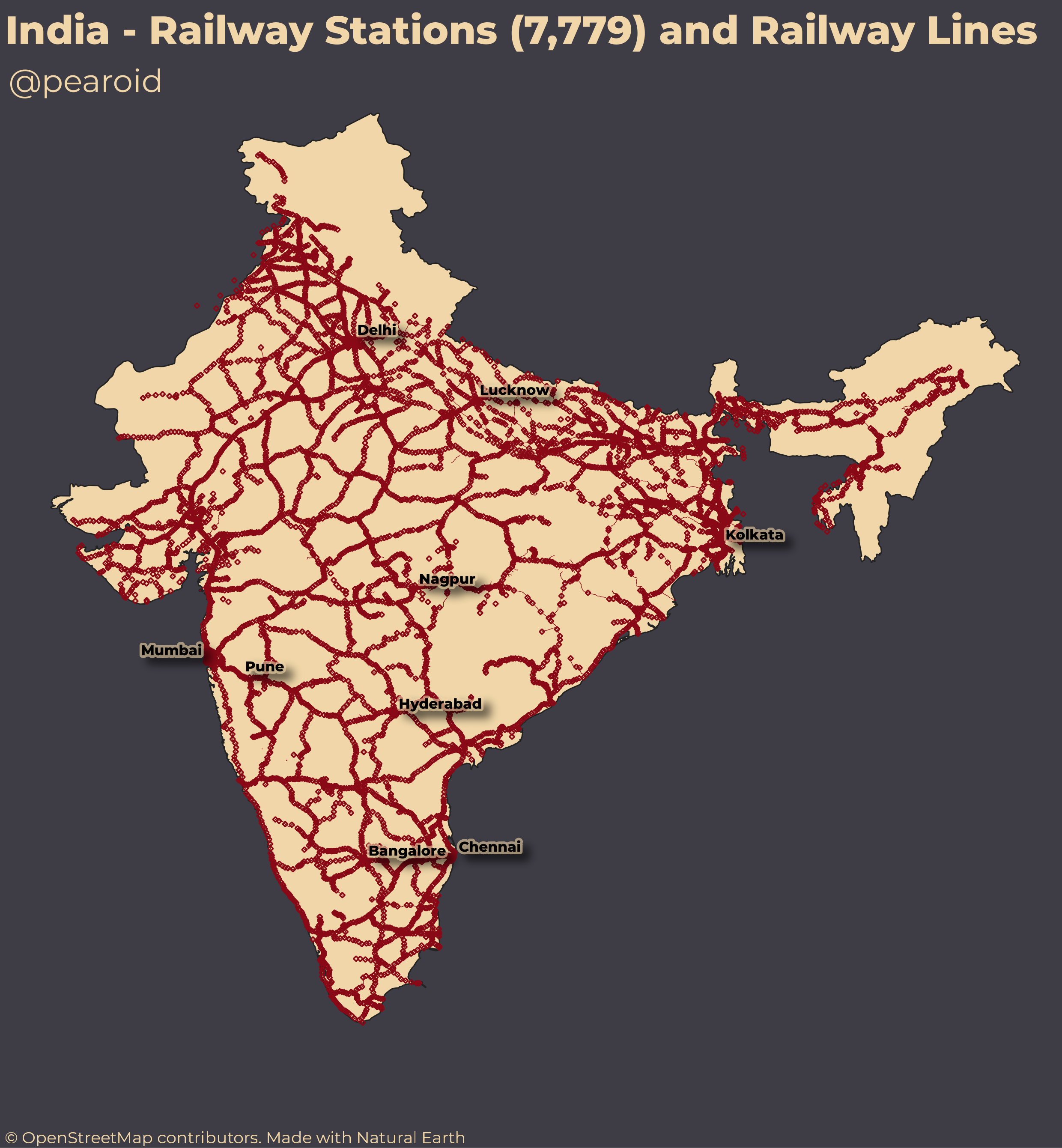
I used the Osmium tool to extract every railway station and line in India and then GDAL to convert them to the geopackage format. The first analysis I undertook was to follow Saroo’s and ascertain how many railway stations are within 1,000km of Howrah railway station. To give some context, OSM has listed 7,979 railway stations and 108,000km of railway line (the Wikipedia page lists 68,155 km (the discrepancy may be accounted for by in the inclusion of every siding and historic railway line etc. in the OSM data). The below map shows every railway station and line from OSM.
To give an idea of Saroo’s methodology of drawing a 1,000km buffer of Kolkata and working outwards that left him with 2,905 to search. Below is a map of all of these.

I decided not to use Saroo’s methodology of using a buffer distance from Kolkata. I had the entire OSM database for India at my disposal so I decided that the first and easiest step to undertake was to find all the railway stations that began with ‘B’ and contained ‘p’, ‘u’ and ‘r’. I used QGIS’s inbuilt python functionality, PyQGIS. I wrote a small script that would use the regular expression module to find stations that matched the above criteria.
import time, re

start = time.time()
# Start Message
print("Program is Starting...")

layer = iface.activeLayer()
prov = layer.dataProvider()

if layer.dataProvider().fieldNameIndex("Relevant_Rail_Stations") == -1:
    layer.dataProvider().addAttributes([QgsField("Criteria_Test", QVariant.String)])
    layer.updateFields()

pattern = '^b.*.[p].*[u].*[r]*$'

# starting layer editing
layer.startEditing()

features = layer.getFeatures()

for feat in features:
    Regex_Stations_Search = feat['name']
    Regex_String = re.compile(pattern, re.IGNORECASE)
    Regex_Match = Regex_String.search(str(Regex_Stations_Search))
    if Regex_Match:
        layer.changeAttributeValue(feat.id(), 11, "Meets_Criteria")
    else:
        layer.changeAttributeValue(feat.id(), 11, "No_Match")

layer.commitChanges()
iface.vectorLayerTools().stopEditing(layer)

end = time.time()

print("Finished running - the program took " + str((round((end - start), 2))) + " seconds")
The above script took 15 seconds to run and it narrowed down the search field from 7,779 to 91 as shown below. I don’t think it is too much of a stretch to take the various ways that he thought it might have been spelled (as below) and to then take the common letters from those spelling and narrow down the search that way.
- Burampour
- Birampur
- Berampur
- Bramapour
- Berampur

Now that we’ve narrowed down the number of possible ‘B’-towns to 91, the next step is to try and use the hometown criteria to find the correct location. We know that Saroo’s hometown had a water tower, river, bridge, dam and a fountain in the park near the station. He believed the town’s name began with ‘G’ and sounded liked ‘Ginestlay’. I could proceed with the other criteria for the ‘B’-town however I felt that with a dam, bridge, river, fountain and water-tower there were enough unique entities that I could try at this stage to find the hometown without dedicating any further resources or time to the ‘B’-town.
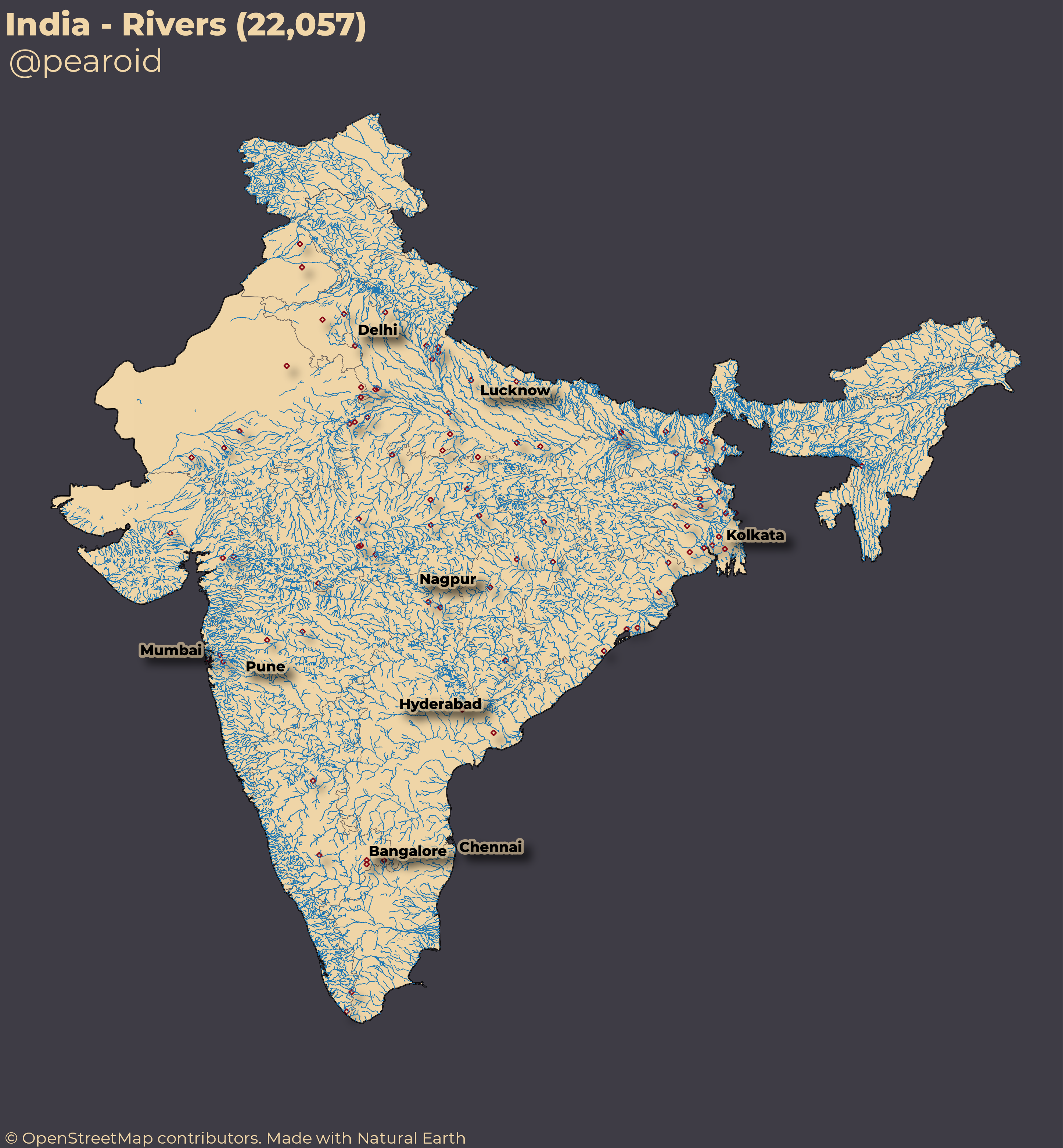
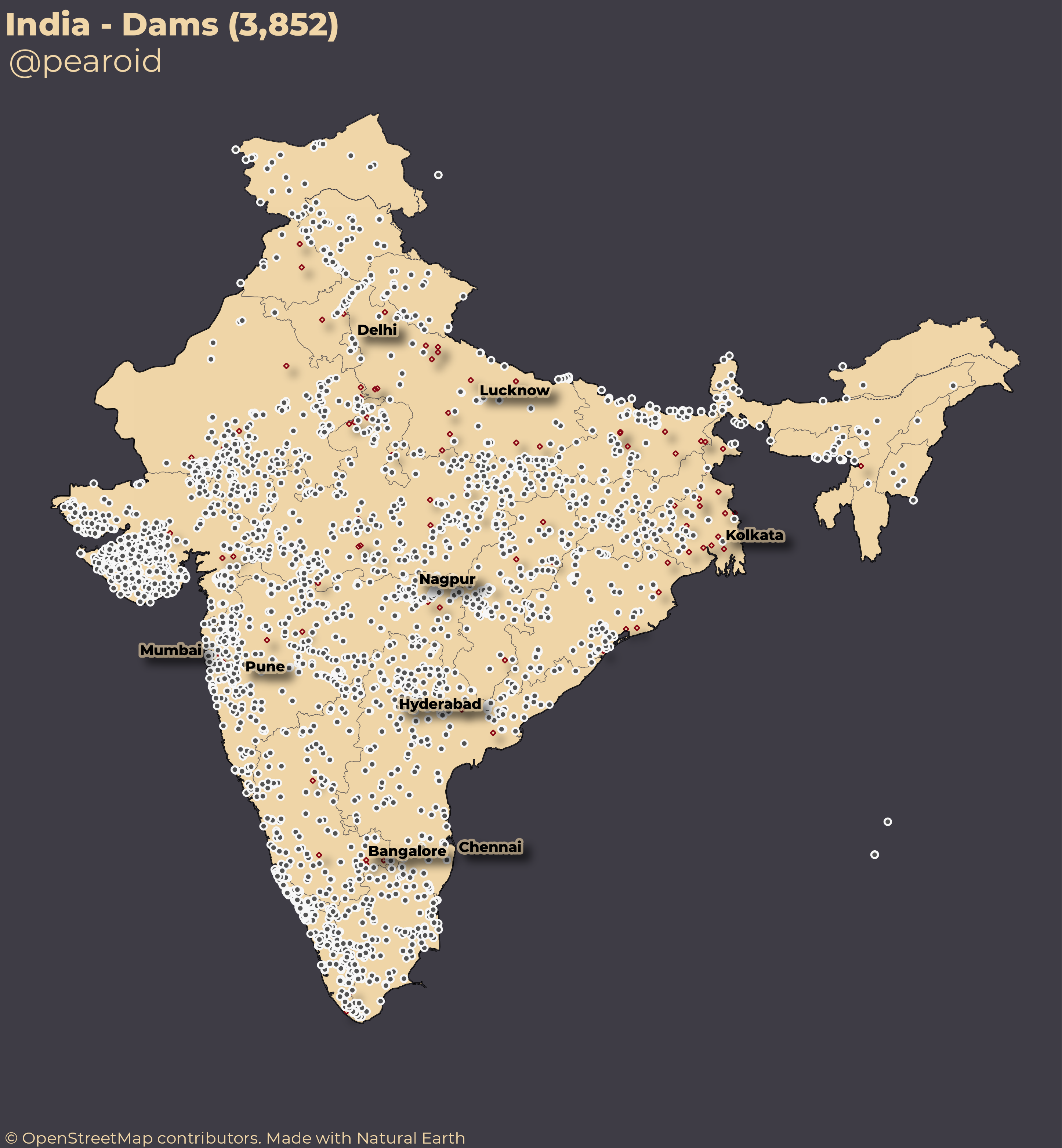
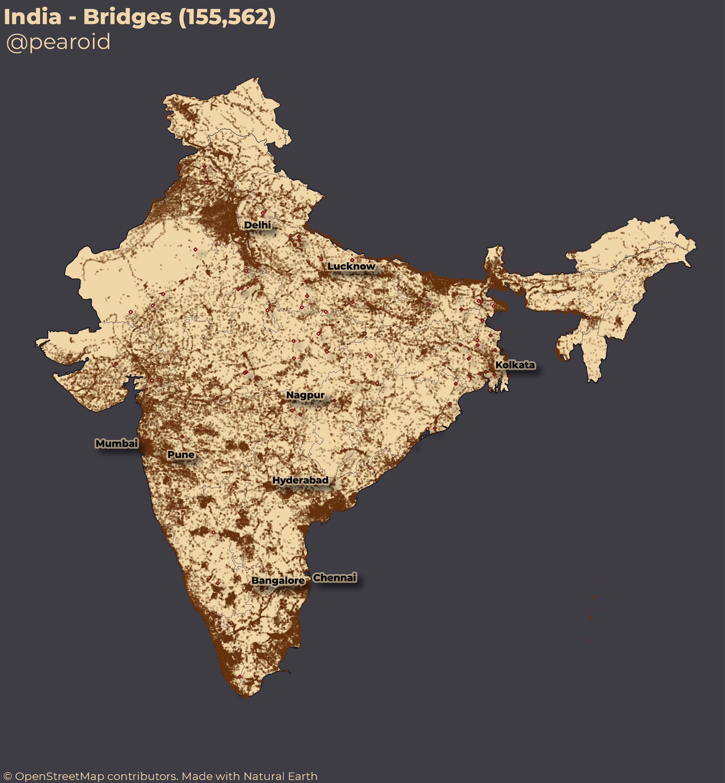
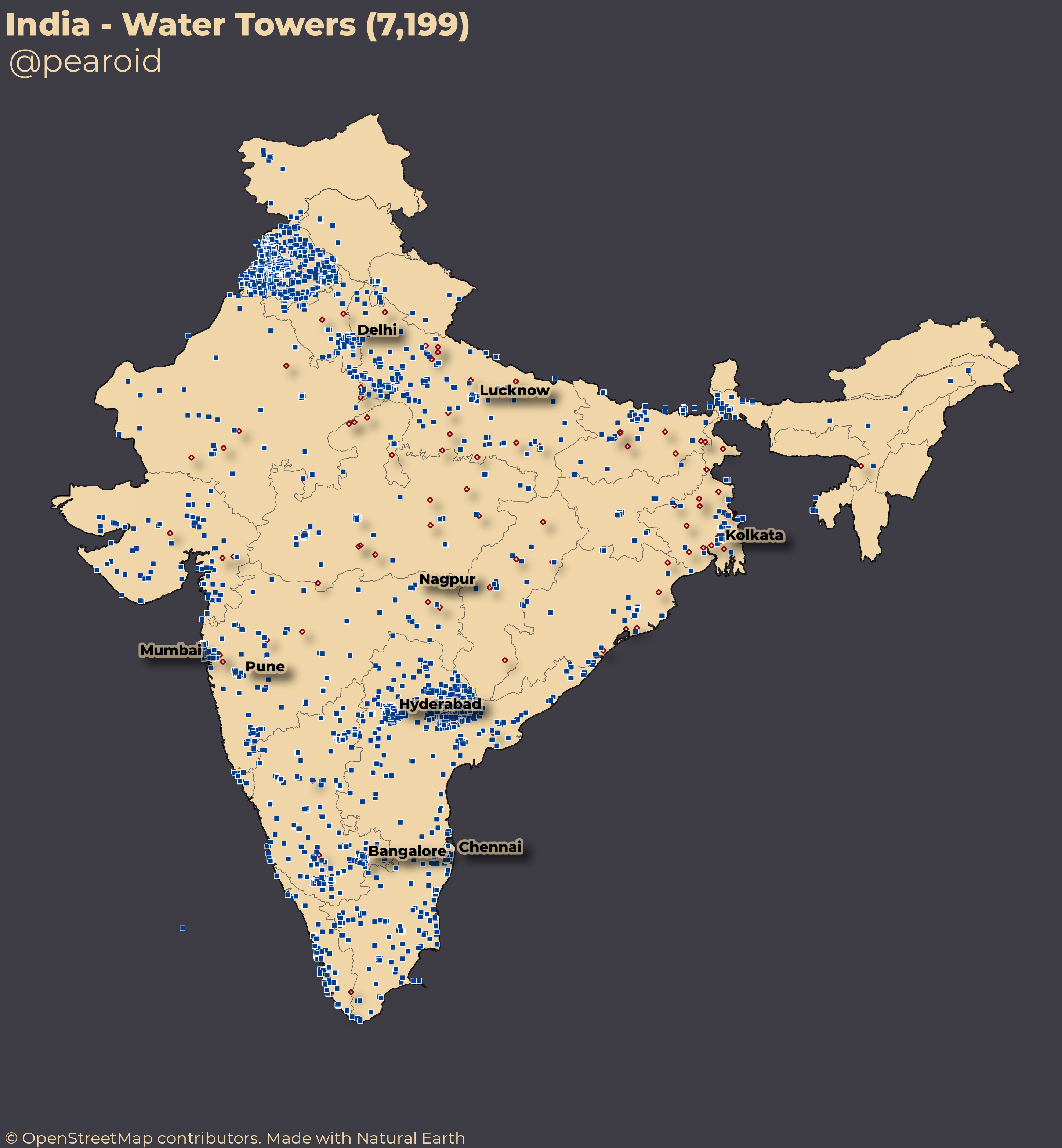
The assumption that Saroo was working on from his friend Amreen’s father was that trains travelled between 70kph-80kph in the mid-80s. As processing power wouldn’t be an issue for what I was trying to do I decided to use the upper limit of 80kph for the speed of the trains. As the PBF file for the entire of India wouldn’t load correctly in QGIS I extracted all of the bridges, dams, rivers and water towers. Below are maps showing the distribution of each from OSM.
I omitted pedestrian over and underpasses at this stage as they were too prevalent to help narrow down the location. I now needed to buffer each of the possible ‘B’-towns by the distance the train would have travelled. Saroo knew that night that Guddu and he travelled for about an hour. I added a small bit of ‘fat’ to my buffer so I used 100km as the buffer distance. I then dissolved the buffers together and clipped them to the coastline. Saroo thought that he been on the train for 12-15 hours. I was thinking that it would be useful to do a buffer from Kolkata of perhaps 6 hours and omit everything inside this buffer as he knew he travelled a farther distance.
A quick GIF of this process is shown below.
Below is the final search area with the every dam, river, bridge, water-tower and train station within 100km of the ‘B’-town stations.
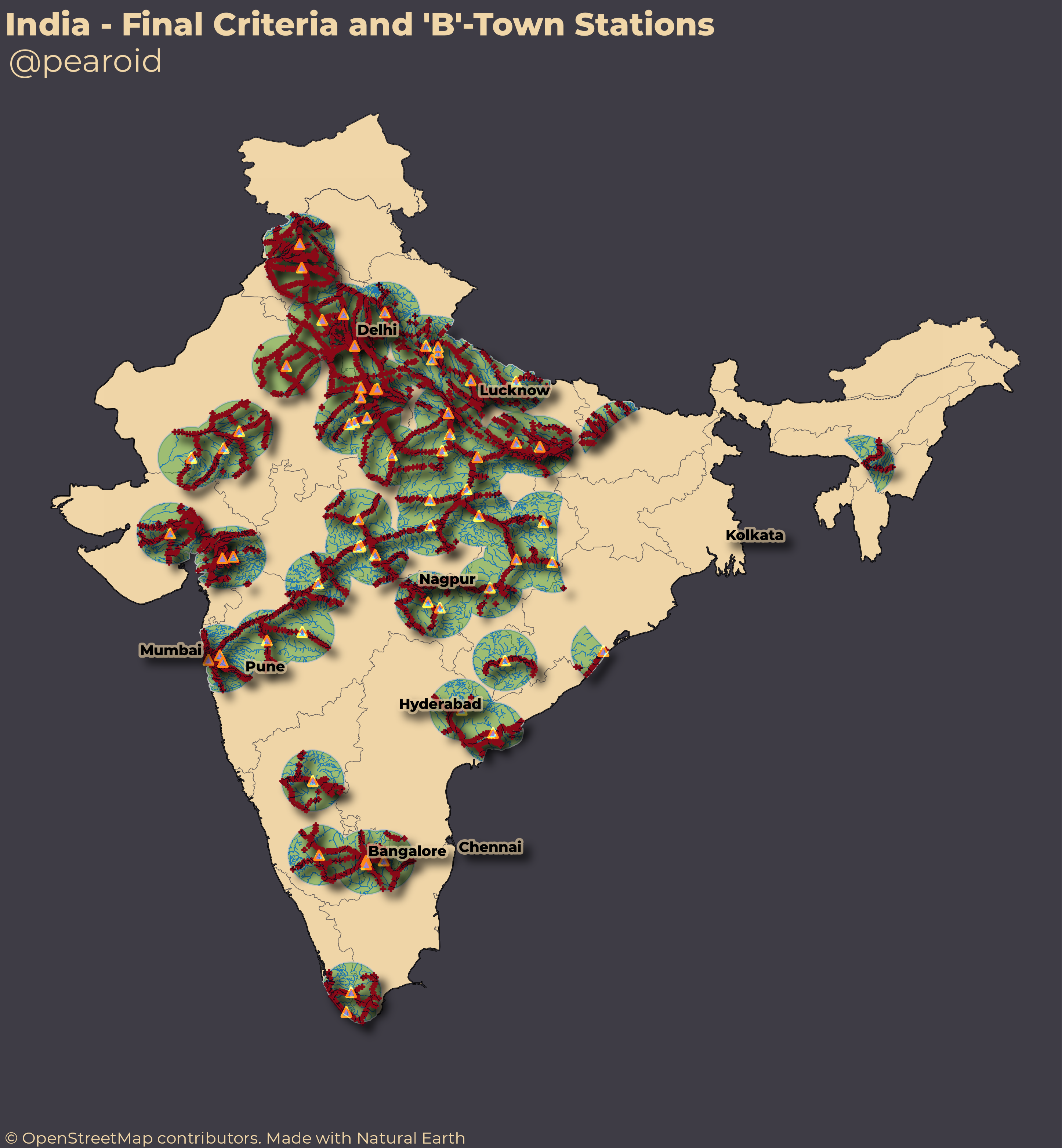
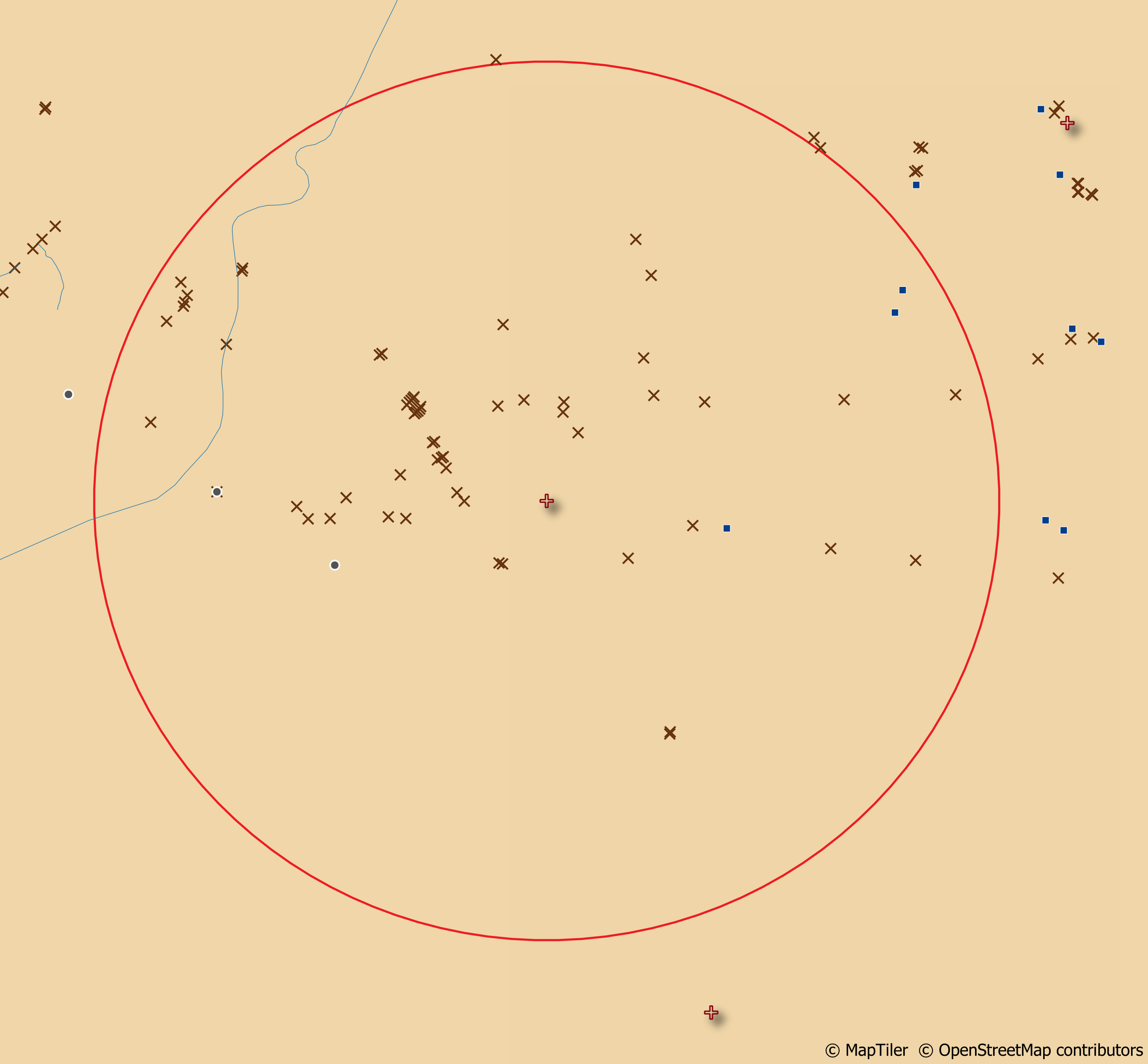
For the final analysis I wanted to find only the stations that had a water-tower, dam, river and bridge within 2km of the station. I picked 2km because I think that would be a reasonable distance for these features to be from a town-centre for 5 year old Saroo to walk to regularly enough to remember them distinctly. We didn’t want to include the ‘B’-town stations themselves so I simply clipped out the data for a distance of 10km from each ‘B’-town as Saroo said that Guddu and him were on the train for about an hour so 10km seems like a safe distance to clip.
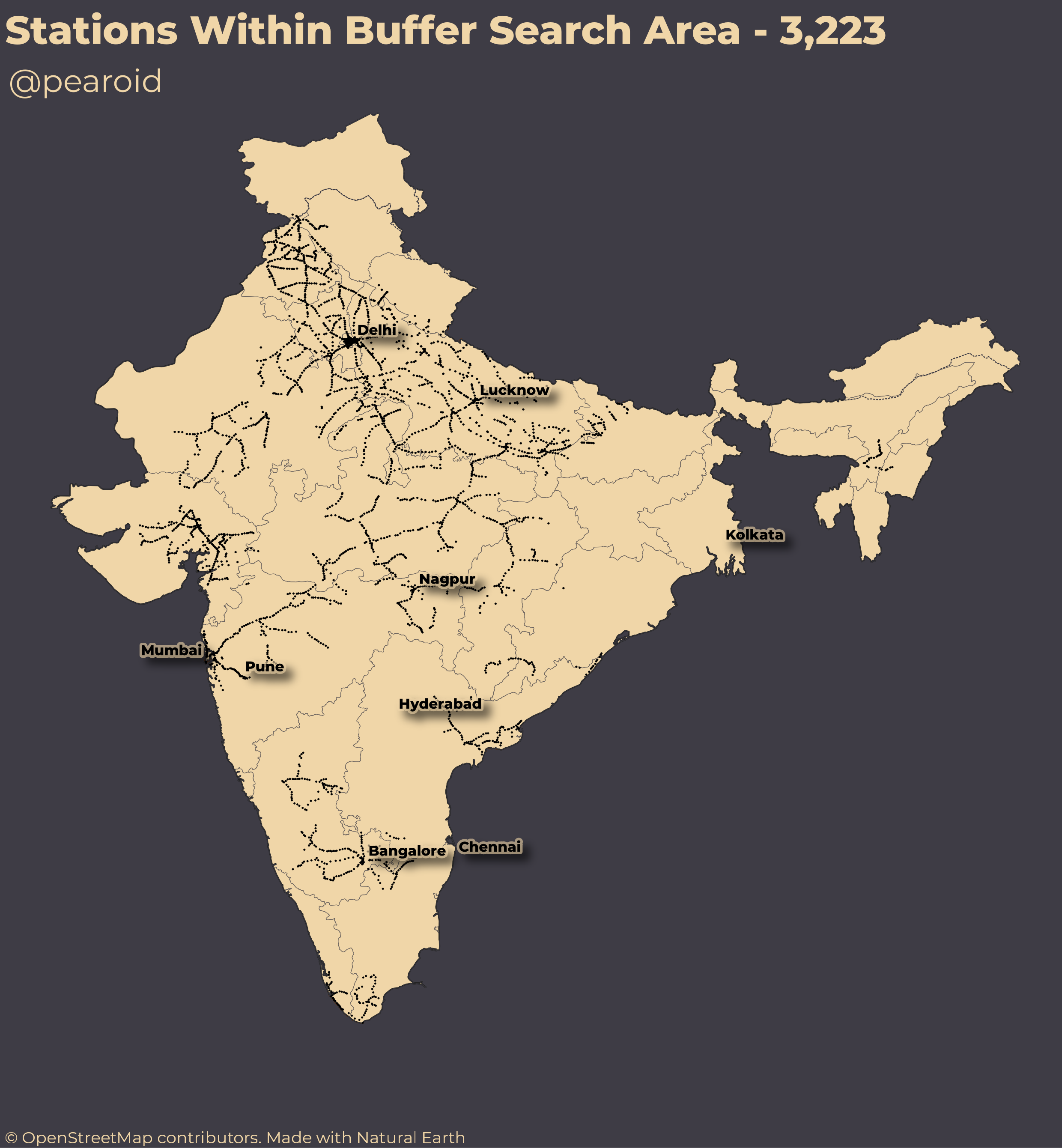
The next step was to find each station that had our relevant criteria within the buffer area. For this I turned to PostGIS (I tried running the query the SQL query in QGIS but it crashed every time). I decided at the first iteration to only use—bridges, water towers and dams as my logic was that these would provide more conclusive than pedestrian over and underpasses and rivers which may have proved too common. Plus, the likelihood of a bridge being for a river was much greater than it being for a ravine, gorge etc. There were 3,223 stations within the 100km buffer of each ‘B’-town station as shown below.
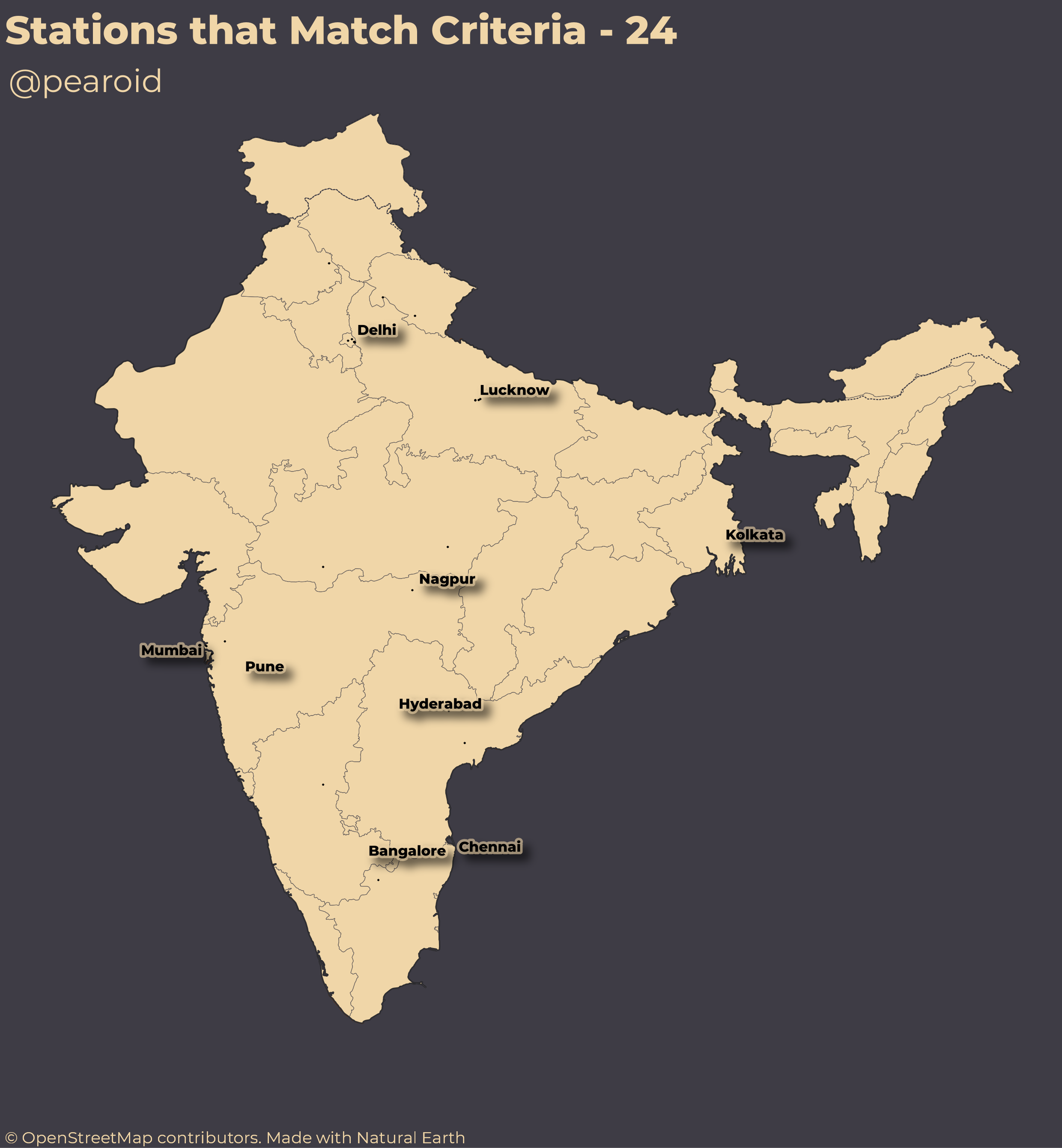
The SQL query that I ran is below, this ran in about a second and returned each station that had a: bridge, water tower or dam within 2km. It narrowed down the number of possible stations from 3,223 to 24 as shown below.
CREATE VIEW Relevant_Stations
AS
SELECT stations_buffered.geom,
     , stations_buffered.name
     , stations_buffered.fid
  FROM stations_buffered
INNER
  JOIN merged_bridge_river_dam
    ON ST_Intersects(stations_buffered.geom, merged_bridge_river_dam.geom)
   AND merged_bridge_river_dam.Feature_Ty IN ('Bridge','DAM','W_Tower')
GROUP
    BY stations_buffered.geom,
     , stations_buffered.name
     , stations_buffered.fid
HAVING COUNT(DISTINCT merged_bridge_river_dam.Feature_Ty) = 3
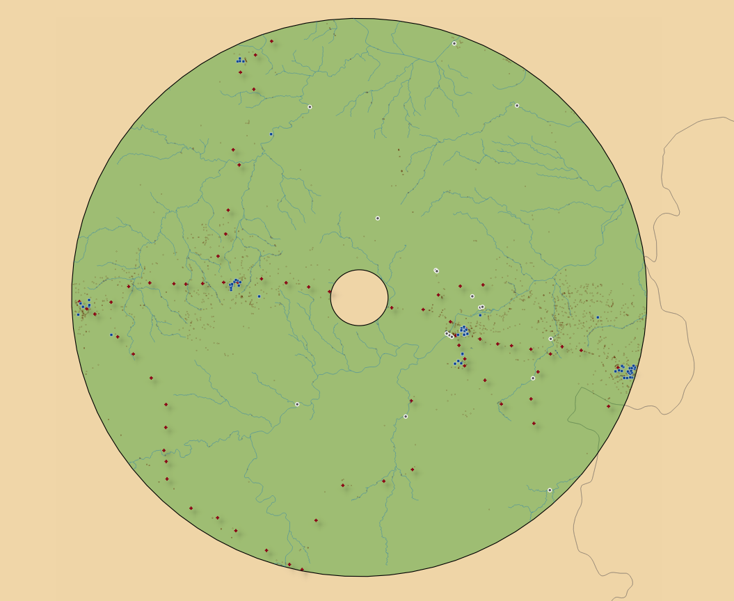
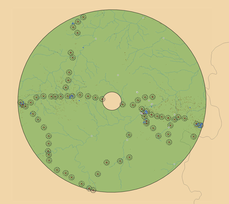
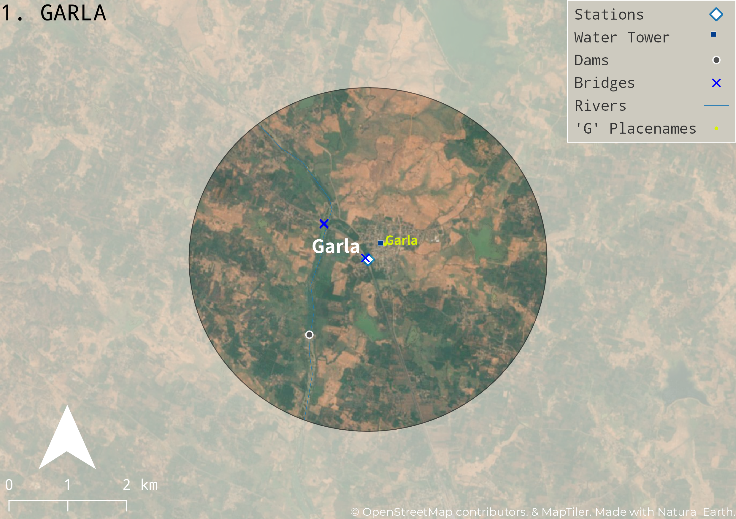
An example of one of the 24 stations that match the criteria is shown below.
Saroo thought that the place he was from sounded like ‘Ginestlay’ so the next step was to find all the OSM tags for ‘place’ that started with ‘G’. I used the below Osmium command to extract all of these place names:
osmium tags-filter india-latest.osm.pbf place=* -o Placenames.osm.pbf
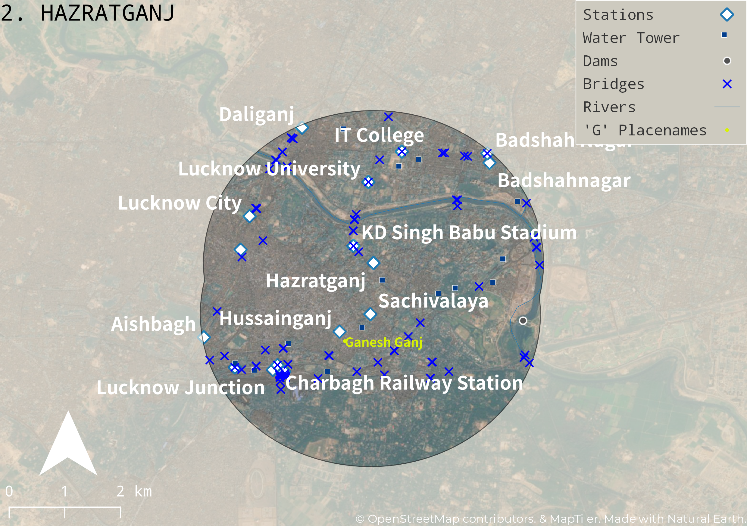
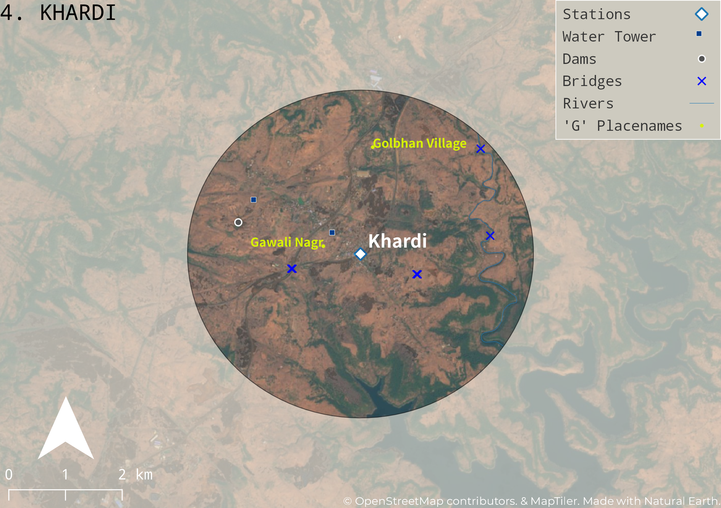
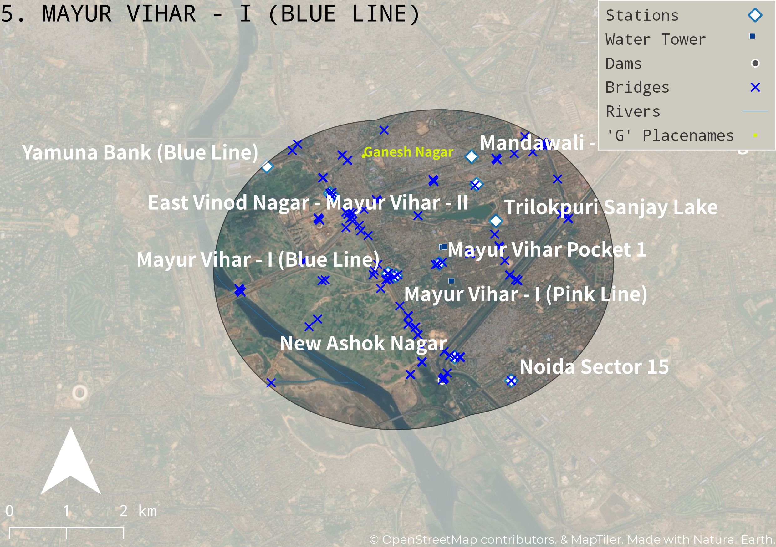
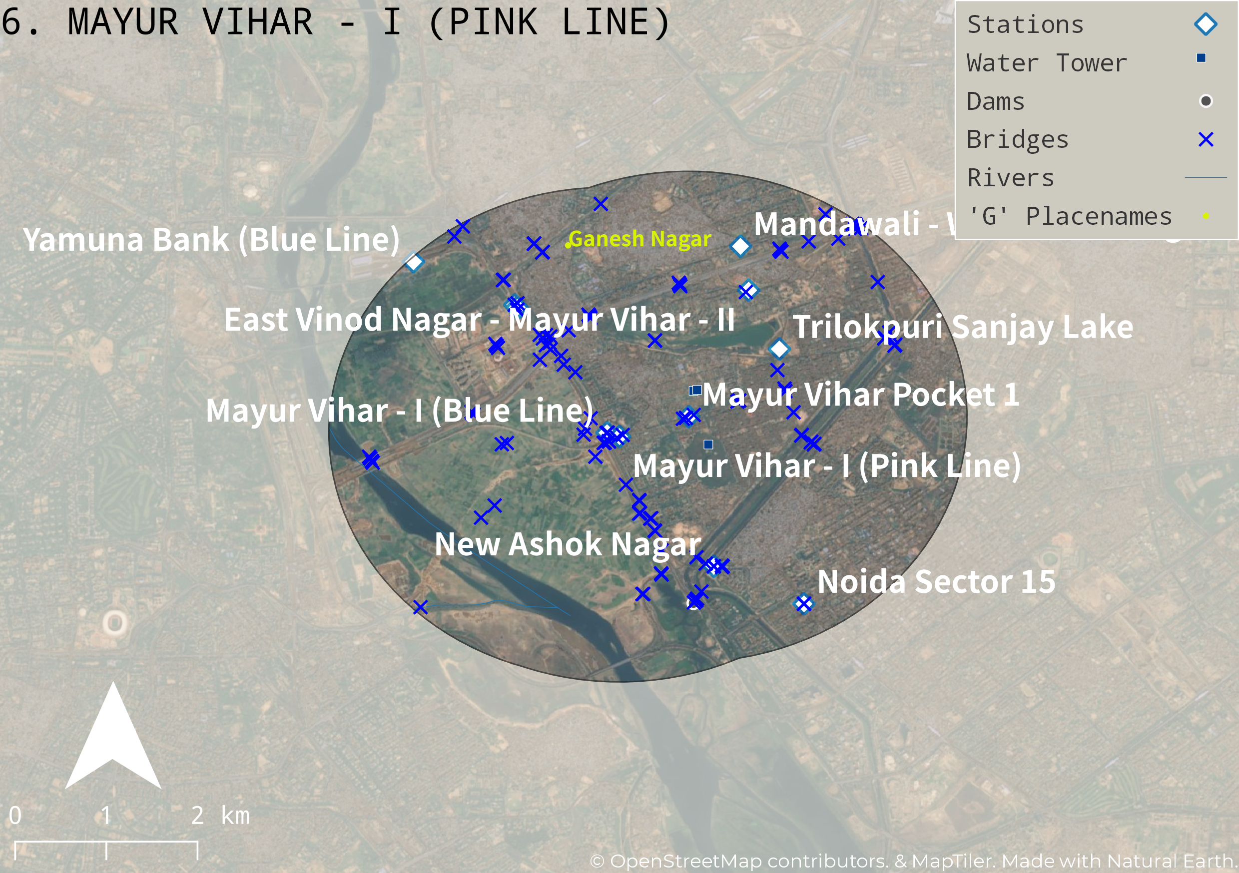
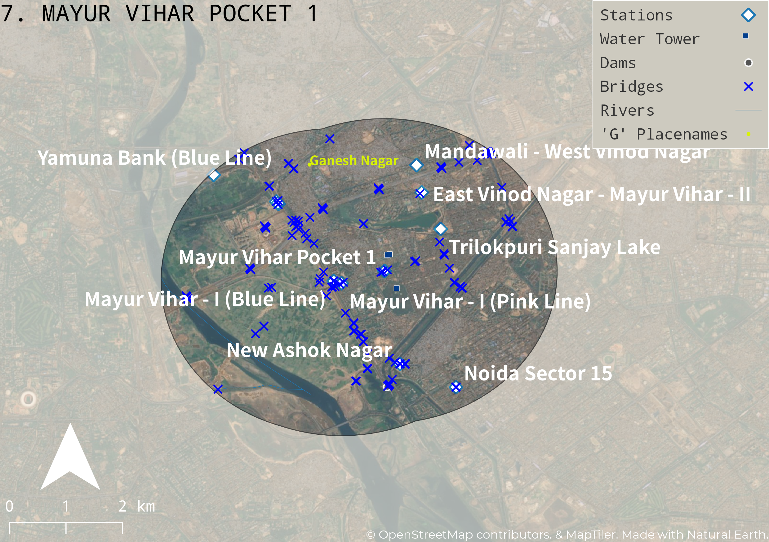
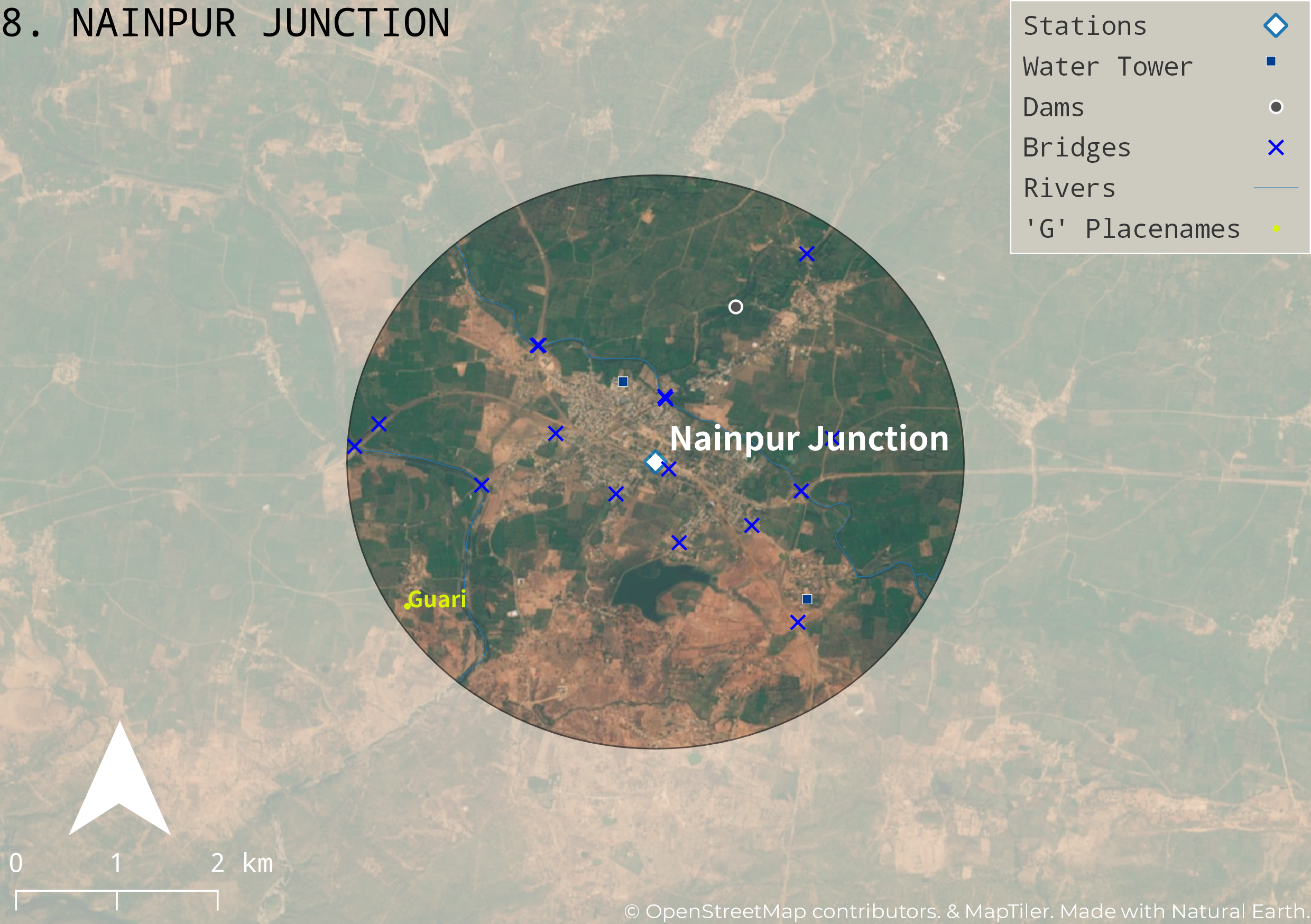
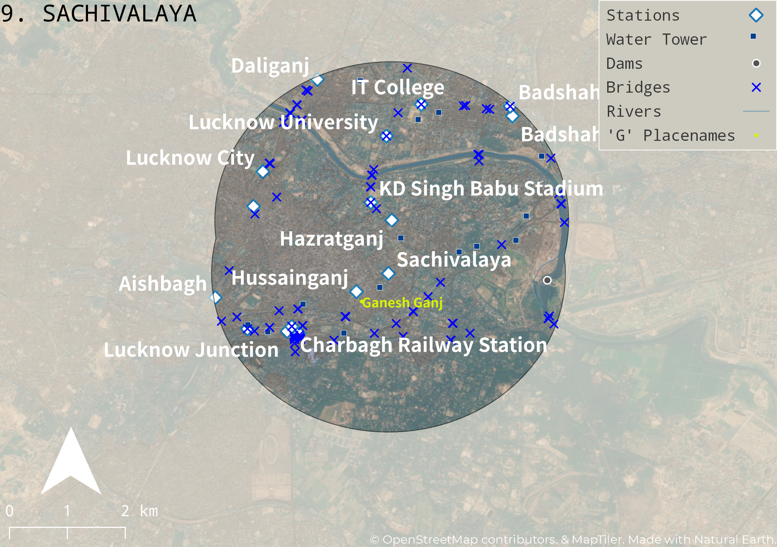
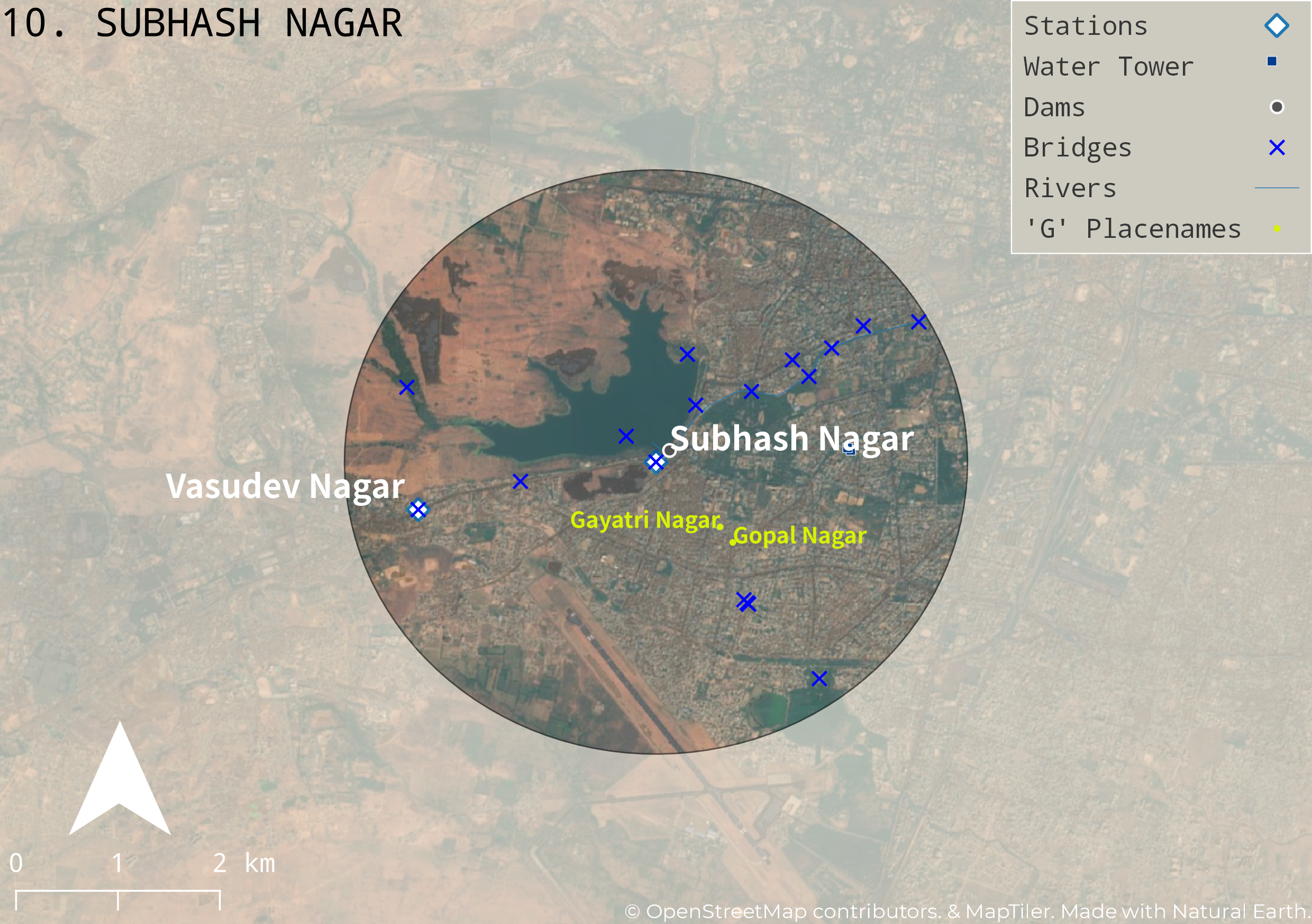
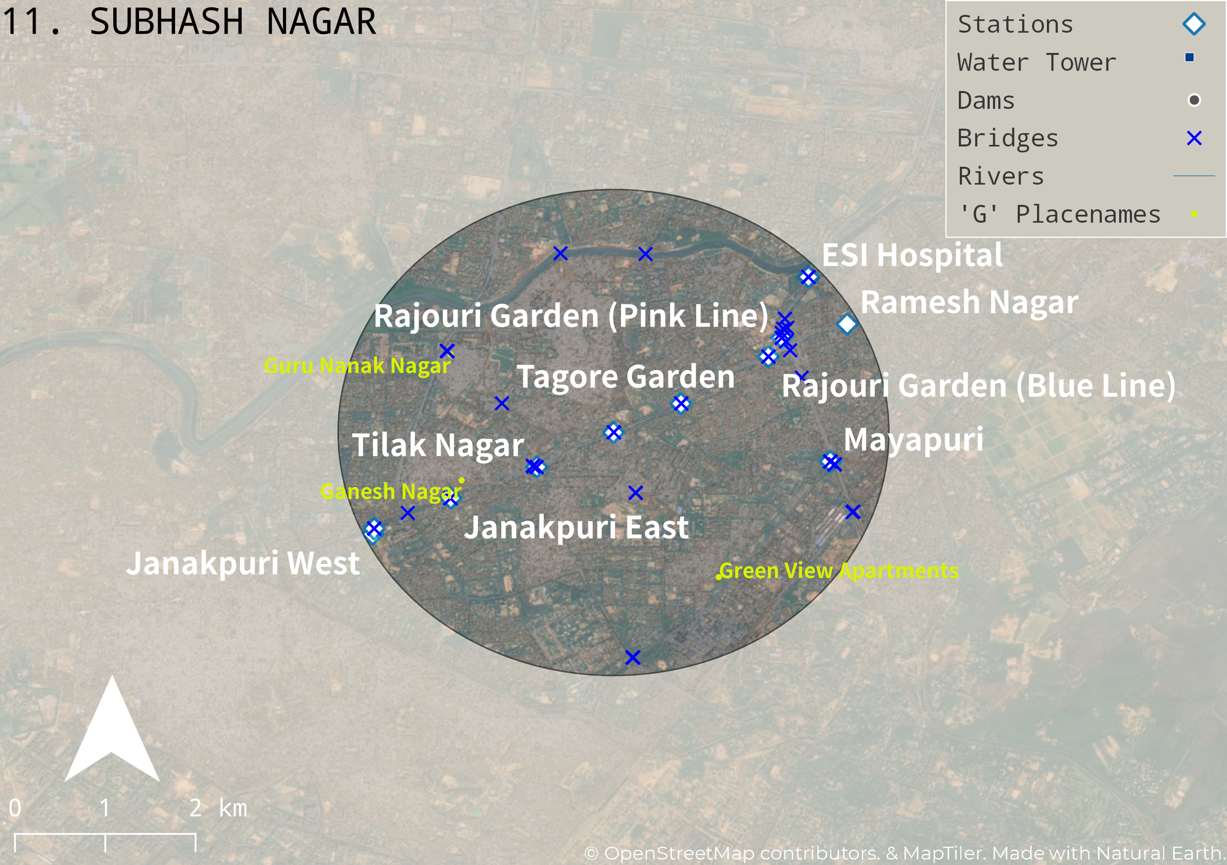
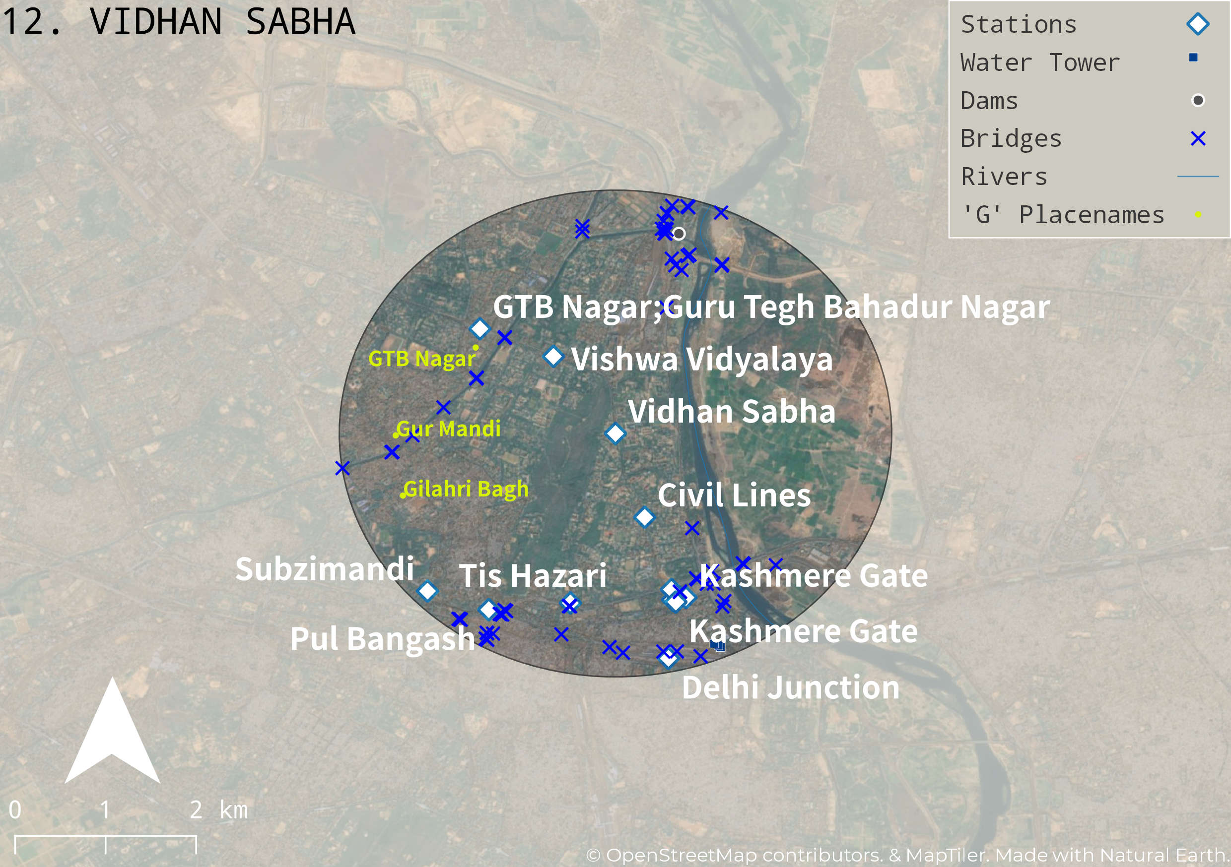
This extracted 193,057 place names for the entire of India. To ensure that I didn’t miss anything I converted the polygons and lines to centroids and merged everything together (this took about 2 minutes in QGIS). I then filtered this by every place that began with ‘G’ and used the ‘Select by Location’ tool to narrow down the list from 24 to 12 stations. I have included images of these 12 stations below. Some of these obviously were not where Saroo was from as they formed parts of large cities (such as Lucknow) but I’ve left them in for the sake of showing the full process.

Conclusion
The station that we were looking for, ‘Khandwa Junction’ with the neighbourhood of ‘Ganesh Talai’ is candidate area 3 above. There are a few observations that I’d like to make regarding the above work. Firstly, I tried to stay as faithful to the criteria that Saroo had to work with. Obviously, I had read the book and I knew the answer. I hope that the above doesn’t feel reverse-engineered. I can honestly say that I didn’t look at any of the OSM data for his hometown prior to starting this post.
I’m conscious of the fact that there is a high likelihood Saroo’s own search along with the media coverage of the movie are the reason the OSM data for Khandwa Junction exists at all. However I will state that all of the above steps are very easily customisable and the criteria easy to change. The parameters could be easily change to test another theory—such as using only a ‘B’ and ‘R’ for the ‘B’-town station perhaps. If we didn’t find the answer we were looking for on the first pass we could have used a DEM to find where train lines crossed a gorge outside of a ‘B’-town station. Or we could have used Python to find all the horseshoe shaped roads outside ‘B’-town stations. Finally, we could have used the data for pedestrian overpasses and underpasses and reran the above.
What I can say with certainly is that with the OSM data available today it was very straightforward to reduce the number of stations to be searched from 2,905 (those within 1,000km of Kolkata) to 12. This would then involve only searching 0.41% of the stations that Saroo originally had to sift through. Google Earth was the best tool available to Saroo at the time but there’s no universe in which it wasn’t a brute-force, sledgehammer to crack a nut tool. I hope with the above work I have shown that it is easy to greatly reduce the number of stations to search through using some decent logic and the power of open-source GIS software and data. I also hope that if anyone else is in a bind similar to Saroo’s that the above might in some way help to demonstrate how to search for the right answer and make it home.